Probability Fundamentals

---

Lecture 03

January 29, 2025

Overview

• Review
• Probability “Review”
• Selecting a Distribution
• Maximum Likelihood
• Describing Uncertainty
• Upcoming Schedule
• References

Review

Null Hypothesis Significance Testing

• Binary “significant”/“non-significant” decision framework;
• Accept or reject null hypothesis \(\mathcal{H}_0\) based on p-value of test statistic (relative to significance level \(\alpha\));
• “Typical” statistical models for \(\mathcal{H}_0\) often chosen out of computational convenience
• There be dragons: Multiple comparisons, lack of statistical power, reading rejection of \(\mathcal{H}_0\) as acceptance of alternative \(\mathcal{H}\)

What NHST Means (and Doesn’t)

• Rejection of \(\mathcal{H}_0\) does not mean \(\mathcal{H}\) is true
• Not rejecting \(\mathcal{H}_0\) does not mean \(\mathcal{H}\) is false.
• Says nothing about \(p(\mathcal{H}_0 | y)\)
• “Simply” a measure of surprise at seeing data under null model.

Probability “Review”

What is Uncertainty?

…A departure from the (unachievable) ideal of complete determinism…

— Walker et al. (2003)

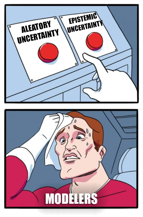
Types of Uncertainty

Uncertainty Type	Source	Example(s)
Aleatory uncertainty	Randomness	Dice rolls, Instrument imprecision
Epistemic uncertainty	Lack of knowledge	Climate sensitivity, Premier League champion

Which Uncertainty Type Meme

Note that the distinction between aleatory and epistemic uncertainty is somewhat arbitrary (aside from maybe some quantum effects). For example, we often think of coin tosses as aleatory, but if we had perfect information about the toss, we might be able to predict the outcome with less uncertainty. There’s a famous paper by Persi Diaconis where he collaborated with engineers to build a device which could arbitrary bias a “fair” coin toss.

But in practice, this doesn’t really matter: the key thing is whether for a given model we’re treating the uncertainty as entirely random (e.g. white noise) versus being interested in the impacts of that uncertainty on the outcome of interest. And there’s a representation theorem by the Bayesian actuary Bruno de Finetti which shows that, under a condition called exchangeability, we can think of any random sequence as arising from an independent and identically distributed process, so the practical difference can collapse further.

Probability

Probability is a language for expressing uncertainty.

The axioms of probability are straightforward:

1. \(\mathcal{P}(E) \geq 0\);
2. \(\mathcal{P}(\Omega) = 1\);
3. \(\mathcal{P}(\cup_{i=1}^\infty E_i) = \sum_{i=1}^\infty \mathcal{P}(E_i)\) for disjoint \(E_i\).

The third is a generalization of the definition of independent events to sets of outcomes.

Frequentist vs Bayesian Probability

Frequentist:

• Probability as frequency over repeated observations.
• Data are random, but parameters are not.
• How consistent are estimates for different data?

Bayesian:

• Probability as degree of belief/betting odds.
• Data and parameters are random variables;
• Emphasis on conditional probability.

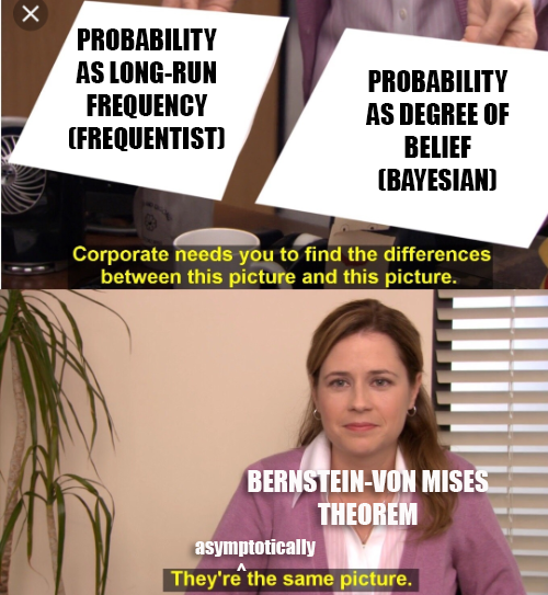
But What, Like, Is Probability?

Frequentist vs. Bayesian: different interpretations with some different methods and formalisms.

We will freely borrow from each school depending on the purpose and goal of an analysis.

Definitions of Probability Meme

Probability Distributions

Distributions are mathematical representations of probabilities over a range of possible outcomes.

\[x \to \mathbb{P}_{\color{green}\mathcal{D}}[x] = p_{\color{green}\mathcal{D}}\left(x | {\color{purple}\theta}\right)\]

• \({\color{green}\mathcal{D}}\): probability distribution (often implicit);
• \({\color{purple}\theta}\): distribution parameters

Sampling Notation

To write \(x\) is sampled from \(\mathcal{D}(\theta) = p(x|\theta)\): \[x \sim \mathcal{D}(\theta)\]

For example, for a normal distribution: \[x \overset{\text{i.i.d.}}{\sim} \mathcal{N}(\mu, \sigma)\]

“i.i.d.” means “identically and independently distributed.””

Probability Density Function

A continuous distribution \(\mathcal{D}\) has a probability density function (PDF) \(f_\mathcal{D}(x) = p(x | \theta)\).

The probability of \(x\) occurring in an interval \((a, b)\) is \[\mathbb{P}[a \leq x \leq b] = \int_a^b f_\mathcal{D}(x)dx.\]

Important: \(\mathbb{P}(x = x^*)\) is zero!

Probability Mass Functions

Discrete distributions have probability mass functions (PMFs) which are defined at point values, e.g. \(p(x = x^*) \neq 0\).

Unlike continuous distributions, we can talk about the probability of individual values for discrete distributions, which a PMF provides versus a PDF. But in general these are the same things.

Cumulative Density Functions

If \(\mathcal{D}\) is a distribution with PDF \(f_\mathcal{D}(x)\), the cumulative density function (CDF) of \(\mathcal{D}\) is \(F_\mathcal{D}(x)\):

\[F_\mathcal{D}(x) = \int_{-\infty}^x f_\mathcal{D}(u)du.\]

(a) Relationship of CDF and PDF

(b)

Figure 1

Relationship Between PDFs and CDFs

Since \[F_\mathcal{D}(x) = \int_{-\infty}^x f_\mathcal{D}(u)du,\]

if \(f_\mathcal{D}\) is continuous at \(x\), the Fundamental Theorem of Calculus gives: \[f_\mathcal{D}(x) = \frac{d}{dx}F_\mathcal{D}(x).\]

The value of the CDF is the amount of probability “below” the value. So e.g. for a one-sided statistical test, the p-value is the complement of the CDF at the value of the test statistic.

Quantiles

The quantile function is the inverse of the CDF:

\[q(\alpha) = F^{-1}_\mathcal{D}(\alpha)\]

So \[x_0 = q(\alpha) \iff \mathbb{P}_\mathcal{D}(X < x_0) = \alpha.\]

(a) Relationship of CDF and PDF

(b)

Figure 2

Selecting a Distribution

Distributions Are Assumptions

Specifying a distribution is making an assumption about observations and any applicable constraints.

Examples: If your observations are…

• Continuous and fat-tailed? Cauchy distribution
• Continuous and bounded? Beta distribution
• Sums of positive random variables? Gamma or Normal distribution.

Why Use a Normal Distribution?

Two main reasons to use linear models/normal distributions:

1. Inferential: “Least informative” distribution assuming knowledge of just mean and variance;
2. Generative: Central Limit Theorem (summed fluctuations are asymptotically normal)

Weight stack Gaussian distribution

Source: r/GymMemes

One key thing: normal distributions are the “least informative” distribution given constraints on mean and variance. So all else being equal, this is a useful machine if all we’re interested in are those two moments.

Statistics of Random Variables are Random Variables

The sum or mean of a random sample is itself a random variable:

\[\bar{X}_n = \frac{1}{n}\sum_{i=1}^n X_i \sim \mathcal{D}_n\]

\(\mathcal{D}_n\): The sampling distribution of the mean (or sum, or other estimate of interest).

Sampling Distributions

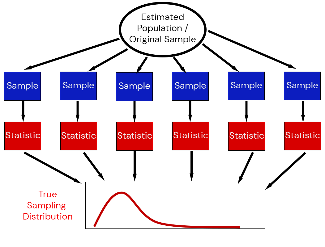
Illustration of the Sampling Distribution

Central Limit Theorem

If

• \(\mathbb{E}[X_i] = \mu\)
• and \(\text{Var}(X_i) = \sigma^2 < \infty\),

\[\begin{align*} &\bbox[yellow, 10px, border:5px solid red] {\lim_{n \to \infty} \sqrt{n}(\bar{X}_n - \mu ) = \mathcal{N}(0, \sigma^2)} \\ \Rightarrow &\bbox[yellow, 10px, border:5px solid red] {\bar{X}_n \overset{\text{approx}}{\sim} \mathcal{N}(\mu, \sigma^2/n)} \end{align*}\]

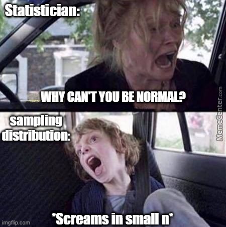
Central Limit Theorem (More Intuitive)

For a large enough set of samples, the sampling distribution of a sum or mean of random variables is approximately a normal distribution, even if the random variables themselves are not.

Small n Meme

Source: Unknown

“What Distribution Should I Use?”

There is no right answer to this, no matter what a statistical test tells you.

• What assumptions are justifiable from theory?
• What information do you have?

“What Distribution Should I Use?”

For example, suppose our data are counts of events:

• If you know something about rates, you can use a Poisson distribution
• If you know something about probabilities, you can use a Binomial distribution.

Q-Q Plots

One exploratory method to see if your data is reasonably described by a theoretical distribution is a Q-Q plot.

samps = rand(Normal(0, 3), 20)
qqplot(Normal, samps, tickfontsize=16, guidefontsize=18, linewidth=3, markersize=6)
xlabel!("Theoretical Quantiles")
ylabel!("Empirical Quantiles")
plot!(size=(500, 450))

Figure 3

Fat-Tailed Data and Q-Q Plots

(a) Normal vs Cauchy Distribution

(b) Q-Q Plot

Figure 4: Q-Q Plot for Cauchy Data and Normal Distribution

Maximum Likelihood

Likelihood

How do we “fit” distributions to a dataset?

Likelihood of data to have come from distribution \(f(\mathbf{x} | \theta)\):

\[\mathcal{L}(\theta | \mathbf{x}) = \underbrace{f(\mathbf{x} | \theta)}_{\text{PDF}}\]

The likelihood gives us a measure of how probable a dataset is from a given distribution. It’s the PDF of the distribution at the data.

But the perspective is flipped: instead of fixing a distribution and calculating the probability of some data, we fix the data and look at how the probability of observing that data changes as the distribution changes.

Normal Distribution PDF

\[f_\mathcal{D}(x) = p(x | \mu, \sigma) = \frac{1}{\sigma\sqrt{2\pi}} \exp\left(-\frac{1}{2}\left(\frac{x - \mu}{\sigma}^2\right)\right)\]

Figure 5

Likelihood of Multiple Samples

For multiple (independent) samples \(\mathbf{x} = \{x_1, \ldots, x_n\}\):

\[\mathcal{L}(\theta | \mathbf{x}) = \prod_{i=1}^n \mathcal{L}(\theta | x_i).\]

Likelihood Example

Distribution	Likelihood
\(N(0, 1)\)	1.9e-8

Likelihood Example

Distribution	Likelihood
\(N(0, 1)\)	1.9e-8
\(N(-1, 2)\)	1.5e-8

Likelihood Example

Distribution	Likelihood
\(N(0, 1)\)	1.9e-8
\(N(-1, 2)\)	1.5e-8
\(N(-1, 1)\)	4.6e-8

Maximizing Likelihood

To find the parameters \(\hat{\theta}\) which best fit the data:

\(\hat{\theta} = \max_\theta \mathcal{L}(\theta | \mathbf{x})\)

Generally Maximizing Likelihood

Can use optimization algorithms to maximize \(\theta \to \mathcal{L}(\theta | x).\)

Dragons: Probability calculations tend to under- and overflow due to floating point precision.

Floating Point Logarithms meme

Describing Uncertainty

Confidence Intervals

Frequentist estimates have confidence intervals, which will contain the “true” parameter value for \(\alpha\)% of data samples.

No guarantee that an individual CI contains the true value (with any “probability”)!

Horseshoe Illustration

Source: https://www.wikihow.com/Throw-a-Horseshoe

Confidence intervals only capture uncertainty in parameter inferences due to data uncertainty, though this language sometimes gets misused to also refer to data/estimand uncertainty.

Example: 95% CIs for N(0.4, 2)

# set up distribution
mean_true = 0.4
n_cis = 100 # number of CIs to compute
dist = Normal(mean_true, 2)

# use sample size of 100
samples = rand(dist, (100, n_cis))
# mapslices broadcasts over a matrix dimension, could also use a loop
sample_means = mapslices(mean, samples; dims=1)
sample_sd = mapslices(std, samples; dims=1) 
mc_sd = 1.96 * sample_sd / sqrt(100)
mc_ci = zeros(n_cis, 2) # preallocate
for i = 1:n_cis
    mc_ci[i, 1] = sample_means[i] - mc_sd[i]
    mc_ci[i, 2] = sample_means[i] + mc_sd[i]
end
# find which CIs contain the true value
ci_true = (mc_ci[:, 1] .< mean_true) .&& (mc_ci[:, 2] .> mean_true)
# compute percentage of CIs which contain the true value
ci_frac1 = 100 * sum(ci_true) ./ n_cis

# plot CIs
p1 = plot([mc_ci[1, :]], [1, 1], linewidth=3, color=:deepskyblue, label="95% Confidence Interval", title="Sample Size 100", yticks=:false, legend=:false)
for i = 2:n_cis
    if ci_true[i]
        plot!(p1, [mc_ci[i, :]], [i, i], linewidth=2, color=:deepskyblue, label=:false)
    else
        plot!(p1, [mc_ci[i, :]], [i, i], linewidth=2, color=:red, label=:false)
    end
end
vline!(p1, [mean_true], color=:black, linewidth=2, linestyle=:dash, label="True Value") # plot true value as a vertical line
xaxis!(p1, "Estimate")
plot!(p1, size=(500, 350)) # resize to fit slide

# use sample size of 1000
samples = rand(dist, (1000, n_cis))
# mapslices broadcasts over a matrix dimension, could also use a loop
sample_means = mapslices(mean, samples; dims=1)
sample_sd = mapslices(std, samples; dims=1) 
mc_sd = 1.96 * sample_sd / sqrt(1000)
mc_ci = zeros(n_cis, 2) # preallocate
for i = 1:n_cis
    mc_ci[i, 1] = sample_means[i] - mc_sd[i]
    mc_ci[i, 2] = sample_means[i] + mc_sd[i]
end
# find which CIs contain the true value
ci_true = (mc_ci[:, 1] .< mean_true) .&& (mc_ci[:, 2] .> mean_true)
# compute percentage of CIs which contain the true value
ci_frac2 = 100 * sum(ci_true) ./ n_cis

# plot CIs
p2 = plot([mc_ci[1, :]], [1, 1], linewidth=3, color=:deepskyblue, label="95% Confidence Interval", title="Sample Size 1,000", yticks=:false, legend=:false)
for i = 2:n_cis
    if ci_true[i]
        plot!(p2, [mc_ci[i, :]], [i, i], linewidth=2, color=:deepskyblue, label=:false)
    else
        plot!(p2, [mc_ci[i, :]], [i, i], linewidth=2, color=:red, label=:false)
    end
end
vline!(p2, [mean_true], color=:black, linewidth=2, linestyle=:dash, label="True Value") # plot true value as a vertical line
xaxis!(p2, "Estimate")
plot!(p2, size=(500, 350)) # resize to fit slide

display(p1)
display(p2)

(a) Sample Size 100

(b) Sample Size 1,000

Figure 6: Display of 95% confidence intervals

95% of the CIs contain the true value (left) vs. 94% (right)

Predictive Intervals

Predictive intervals capture uncertainty in an estimand.

With what probability would I see a particular outcome in the future?

Often need to construct these using simulation.

Figure 7: Two different 95% credible intervals.

Due to this non-uniqueness, the typical convention is to use the “equal tailed” interval based on quantiles.

Upcoming Schedule

Next Classes

Next Week: Probability Models for Data

Assessments

Homework 1 due next Friday (2/7).

Quiz: Due before next class.

Reading: Annotate/submit writing before next class, will reserve time for discussion.

References

References (Scroll for Full List)

Walker, W. E., Harremoës, P., Rotmans, J., Sluijs, J. P. van der, Asselt, M. B. A. van, Janssen, P., & Krayer von Krauss, M. P. (2003). Defining uncertainty: A conceptual basis for uncertainty management in model-based decision support. Integrated Assessment, 4, 5–17. https://doi.org/10.1076/iaij.4.1.5.16466