Probability Models
Lecture 04
February 3, 2024
Review
Probability Fundamentals
- Bayesian vs. Frequentist Interpretations
- Distributions reflect assumptions on probability of data.
- Normal distributions: “least informative” distribution for a given mean/variance.
- Fit distributions by maximizing likelihood.
- Communicating uncertainty: confidence vs. predictive intervals.
Linear Regression
How Does River Flow Affect TDS?
Question: Does river flow affect the concentration of total dissolved solids?
Data: Cuyahoga River (1969 – 1973), from Helsel et al. (2020, Chapter 9).
How Does TDS Affect River Flow?
Question: Does river flow affect the concentration of total dissolved solids?
Model: \[D \rightarrow S \ {\color{purple}\leftarrow U}\] \[S = f(D, U)\]
Log-Linear Relationships
\[ \begin{align*} S &= \beta_0 + \beta_1 \log(D) + U\\ U &\sim \mathcal{N}(0, \sigma^2) \end{align*} \]
Likelihood
How do we find \(\beta_i\) and \(\sigma\)?
Likelihood of data to have come from distribution \(f(\mathbf{x} | \theta)\): \[\mathcal{L}(\theta | \mathbf{x}) = \underbrace{f(\mathbf{x} | \theta)}_{\text{PDF}}\]
Here the randomness comes from \(U\): \[S \sim \mathcal{N}(\beta_0 + \beta_1 \log(D), \sigma^2)\]
Maximizing Gaussian Likelihood ⇔ Least Squares
\[y_i \sim \mathcal{N}(F(x_i), \sigma^2)\]
\[\mathcal{L}(\theta | \mathbf{y}; F) = \prod_{i=1}^n \frac{1}{\sqrt{2\pi}} \exp(-\frac{y_i - F(x_i)^2}{2\sigma^2})\]
\[\log \mathcal{L}(\theta | \mathbf{y}; F) = \sum_{i=1}^n \left[\log \frac{1}{\sqrt{2\pi}} - \frac{1}{2\sigma^2}(y_i - F(x_i))^2 \right]\]
\[ \begin{align} \log \mathcal{L}(\theta | \mathbf{y}, F) &= \sum_{i=1}^n \left[\log \frac{1}{\sqrt{2\pi}} - \frac{1}{2\sigma^2}(y_i - F(x_i)) ^2 \right] \\ &= n \log \frac{1}{\sqrt{2\pi}} - \frac{1}{2\sigma^2} \sum_{i=1}^n (y_i - F(x_i))^2 \end{align} \]
Ignoring constants (including \(\sigma\)):
\[\log \mathcal{L}(\theta | \mathbf{y}, F) \propto -\sum_{i=1}^n (y_i - F(x_i))^2.\]
Maximizing \(f(x)\) is equivalent to minimizing \(-f(x)\):
\[ -\log \mathcal{L}(\theta | \mathbf{y}, F) \propto \sum_{i=1}^n (y_i - F(x_i))^2 = \text{MSE} \]
But note: Don’t get an estimate of \(\sigma^2\) directly through least squares.
Back to the Problem…
# tds_riverflow_loglik: function to compute the log-likelihood for the tds model
# θ: vector of model parameters (coefficients β₀ and β₁ and stdev σ)
# tds, flow: vectors of data
function tds_riverflow_loglik(θ, tds, flow)
    β₀, β₁, σ = θ # unpack parameter vector
    μ = β₀ .+ β₁ * log.(flow) # find mean
    ll = sum(logpdf.(Normal.(μ, σ), tds)) # compute log-likelihood
    return ll
end

lb = [0.0, -1000.0, 1.0]
ub = [1000.0, 1000.0, 100.0]
θ₀ = [500.0, 0.0, 50.0]
optim_out = Optim.optimize(θ -> -tds_riverflow_loglik(θ, tds.tds_mgL, tds.discharge_cms), lb, ub, θ₀)
θ_mle = round.(optim_out.minimizer; digits=0)
@show θ_mle;
θ_mle = [610.0, -112.0, 72.0]Maximum Likelihood Results
# simulate 10,000 predictions
x = 1:0.1:60
μ = θ_mle[1] .+ θ_mle[2] * log.(x)

y_pred = zeros(length(x), 10_000)
for i = 1:length(x)
    y_pred[i, :] = rand(Normal(μ[i], θ_mle[3]), 10_000)
end
# take quantiles to find prediction intervals
y_q = mapslices(v -> quantile(v, [0.05, 0.5, 0.95]), y_pred; dims=2)

plot(p1,
    x,
    y_q[:, 2],
    ribbon = (y_q[:, 2] - y_q[:, 1], y_q[:, 3] - y_q[:, 2]),
    linewidth=3,
    fillalpha=0.2,
    label="Best Fit",
    size=(600, 550))
Residual Analysis
More General Models
Structure of a Probability Model
Unpacking linear regression:
\[\begin{align*} y_i &\sim N(\mu_i, \sigma^2) \\ \mu_i &= \sum_j \beta_j x^j_i \end{align*} \]
Note: Can handle heteroskedastic errors with a regression \[\sigma_i^2 = \sum_j \alpha_j z^j_i\]
Think Generatively
Components of probability model for observations:
- Model for “system state” (LR: \(\sum_j \beta_j x^j_i\))
- Choice of “error” distribution (LR: \(N(0, \sigma^2)\))
Source: Richard McElreath
You Can Always Fit Models…
But not all models are theoretically justifiable.

How Do We Choose What To Model?
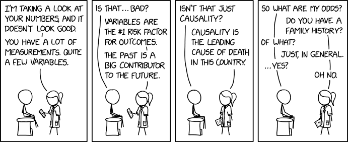
XKCD 2620
Source: XKCD 2620
Example: Modeling Counts
What Distribution?
Count data can be modeled using a Poisson or negative binomial distribution.
Exploring the Data
- Mean: 3.3
- Variance: 135.4
Model Specification
We might hypothesize that more people fishing for more hours results in a greater chance of catching fish.
\[\begin{align*} y_i &\sim Poisson(\lambda_i) \\ f(\lambda_i) &= \beta_0 + \beta_1 P_i + \beta_2 H_i \end{align*} \]
\(\lambda_i\): positive “rate”
\(f(\cdot)\): maps positive reals (rate scale) to all reals (linear model scale)
Link Functions
\(\color{brown}f\) is the link function.
\(\color{royalblue}f^{-1}\) is the inverse link.
\[\begin{align*} y_i &\sim Poisson(\lambda_i) \\ {\color{brown}f}(\lambda_i) &= \beta_0 + \beta_1 P_i + \beta_2 H_i \end{align*} \]
\[ \lambda_i = {\color{royalblue}f^{-1}}\left(\beta_0 + \beta_1 P_i + \beta_2 H_i\right) \]
Choosing a Link Function
Link functions are typically linked to distributions.
- Poisson models usually use the log link (positives → reals).
- Binomial/Bernoulli models use the logit link (\([0, 1]\) → reals) \[\text{logit}(p) = \log\left(\frac{p}{1-p}\right)\]
Fitting the Model
function fish_model(params, persons, hours, fish_caught)
    β₀, β₁, β₂ = params
    λ = exp.(β₀ .+ β₁ * persons + β₂ * hours)
    loglik = sum(logpdf.(Poisson.(λ), fish_caught))
end

lb = [-100.0, -100.0, -100.0]
ub = [100.0, 100.0, 100.0]
init = [0.0, 0.0, 0.0]

optim_out = optimize(θ -> -fish_model(θ, fish.persons, fish.hours, fish.fish_caught), lb, ub, init)
θ_mle = optim_out.minimizer
@show round.(θ_mle; digits=1);
round.(θ_mle; digits = 1) = [-1.5, 0.8, 0.0]Evaluating Model Fit
What Was The Problem?
- Model neglected other plausible contributors, e.g. live bait.
- Data is over-dispersed: higher variance than mean.
- Might be better described by a zero-inflated Poisson model:
- Visitors who spent little time are likely to catch no fish.
- Visitors who spent more time are likely to catch positive fish.
Key Points
Probability Models
- Think of regression as modeling system state (or expectation).
- Full probability model includes distribution of “errors” from expected state.
- Error models can be complex! More on this later…
- Generalized linear models may require a link to map regression to parameters.
- Fit models by maximizing likelihood: no problem using optimization routines.
Upcoming Schedule
Next Classes
Wednesday: Modeling Time Series
Next Week: Bayesian Statistics and Inference
Assessments
Homework 1 Due Friday (2/7).
References
References (Scroll for Full List)
Helsel, D. R., Hirsch, R. M., Ryberg, K. R., Archfield, S. A., & Gilroy, E. J. (2020). Statistical methods in water resources (research report No. 4-A3) (p. 484). Reston, VA: U.S. Geological Survey. Retrieved from http://pubs.er.usgs.gov/publication/tm4A3