Time Series

Lecture 05

February 5, 2025

Time Series

Time Series and Environmental Data

Many environmental datasets involve time series: repeated observations over time:

\[X = \{X_t, X_{t+h}, X_{t+2h}, \ldots, X_{t+nh}\}\]

More often: ignore sampling time in notation,

\[X = \{X_1, X_2, X_3, \ldots, X_n\}\]

Figure 1: Example of time series; trapped lynx populations in Canada.

When Do We Care About Time Series?

Dependence: History or sequencing of the data matters

\[p(y_t) = f(y_1, \ldots, y_{t-1})\]

Serial dependence captured by autocorrelation:

\[\varsigma(i) = \rho(y_t, y_{t-i}) = \frac{\text{Cov}[y_t, y_{t+i}]}{\mathbb{V}[y_t]} \]

Figure 2: Autocorrelation for the Lynx data.

Stationarity

I.I.D. Data: All data drawn from the same distribution, \(y_i \sim \mathcal{D}\).

Equivalent for time series \(\mathbf{y} = \{y_t\}\) is stationarity.

Strict stationarity: \(\{y_t, \ldots, y_{t+k-1}\} \sim \mathcal{D}\) for all \(t\).
Weak stationarity: \(\mathbb{E}[X_1] = \mathbb{E}[X_t]\) and \(\text{Cov}(X_1, X_k) = \text{Cov}(X_t, X_{t+k-1})\) for all \(t\).

Stationary vs. Non-Stationary Series

(a) Stationary vs. Non-stationary time series

(b)

Figure 3

Autocorrelation

(a) Lag-1 autocorrelation for an AR model and Gaussian noise.

(b)

(c)

(d)

Figure 4

Autoregressive (AR) Models

AR(p): (autoregressive of order \(p\)):

\[ \begin{align*} y_t &= \sum_{i=1}^p \rho_{i} y_{t-i} + \varepsilon \\ \varepsilon &\sim N(0, \sigma^2) \end{align*} \]

e.g. AR(1):

\[ \begin{align*} y_t &= \rho y_{t-1} + \varepsilon \\ \varepsilon &\sim N(0, \sigma^2) \end{align*} \]

Uses of AR Models

AR models are commonly used for prediction: bond yields, prices, electricity demand, short-run weather.

But may have little explanatory power: what causes the autocorrelation?

AR(1) Models

(a) AR(1) model

(b)

Figure 5

Diagnosing Autocorrelation

Plot \(\varsigma(i)\) over a series of lags.

Data generated by an AR(1) with \(\rho = 0.7\).

Note: Even without an explicit dependence between \(y_{t-2}\) and \(y_t\), \(\varsigma(2) \neq 0\).

Figure 6: Autocorrelation Function

Partial Autocorrelation

Instead, can isolate \(\varsigma(i)\) independent of \(\varsigma(i-k)\) through partial autocorrelation.

Typically estimated through regression.

Figure 7: Partial autocorrelation Function

AR(1) and Stationarity

\[\begin{align*} y_{t+1} &= \rho y_t + \varepsilon_t \\ y_{t+2} &= \rho^2 y_t + \rho \varepsilon_t + \varepsilon_{t+1} \\ y_{t+3} &= \rho^3 y_t + \rho^2 \varepsilon_t + \rho \varepsilon_{t+1} + \varepsilon_{t+2} \\ &\vdots \end{align*} \]

Under what condition will \(\mathbf{y}\) be stationary?

Stationarity requires \(| \rho | < 1\).

AR(1) Variance

The conditional variance \(\mathbb{V}[y_t | y_{t-1}] = \sigma^2\).

Unconditional variance for stationary \(\mathbb{V}[y_t]\):

\[ \begin{align*} \mathbb{V}[y_t] &= \rho^2 \mathbb{V}[y_{t-1}] + \mathbb{V}[\varepsilon] \\ &= \rho^2 \mathbb{V}[y_t] + \sigma^2 \\ &= \frac{\sigma^2}{1 - \rho^2}. \end{align*} \]

AR(1) Joint Distribution

Assume stationarity and zero-mean process.

Need to know \(\text{Cov}[y_t, y_{t+h}]\) for arbitrary \(h\).

\[ \begin{align*} \text{Cov}[y_t, y_{t-h}] &= \text{Cov}[\rho^h y_{t-h}, y_{t-h}] \\ &= \rho^h \text{Cov}[y_{t-h}, y_{t-h}] \\ &= \rho^h \frac{\sigma^2}{1-\rho^2} \end{align*} \]

AR(1) Joint Distribution

\[ \begin{align*} \mathbf{y} &\sim \mathcal{N}(\mathbf{0}, \Sigma) \\ \Sigma &= \frac{\sigma^2}{1 - \rho^2} \begin{pmatrix}1 & \rho & \ldots & \rho^{T-1} \\ \rho & 1 & \ldots & \rho^{T-2} \\ \vdots & \vdots & \ddots & \vdots \\ \rho^{T-1} & \rho^{T-2} & \ldots & 1\end{pmatrix} \end{align*} \]

Alternatively..

An often “easier approach” (often more numerically stable) is to whiten the series sample/compute likelihoods in sequence:

\[ \begin{align*} y_1 & \sim N\left(0, \frac{\sigma^2}{1 - \rho^2}\right) \\ y_t &\sim N(\rho y_{t-1} , \sigma^2) \end{align*} \]

Dealing with Trends

\[y_t = \underbrace{x_t}_{\text{fluctuations}} + \underbrace{z_t}_{\text{trend}}\]

Model trend with regression: \[y_t - a - bt \sim N(\rho (y_{t-1} - a - bt), \sigma^2)\]
Model the spectrum (frequency domain).
Difference values: \(\hat{y}_t = y_t - y_{t-1}\)

Be Cautious with Detrending!

Dragons: Extrapolating trends identified using “curve-fitting” is highly fraught, complicating projections.

Better to have an explanatory model (next week!)…

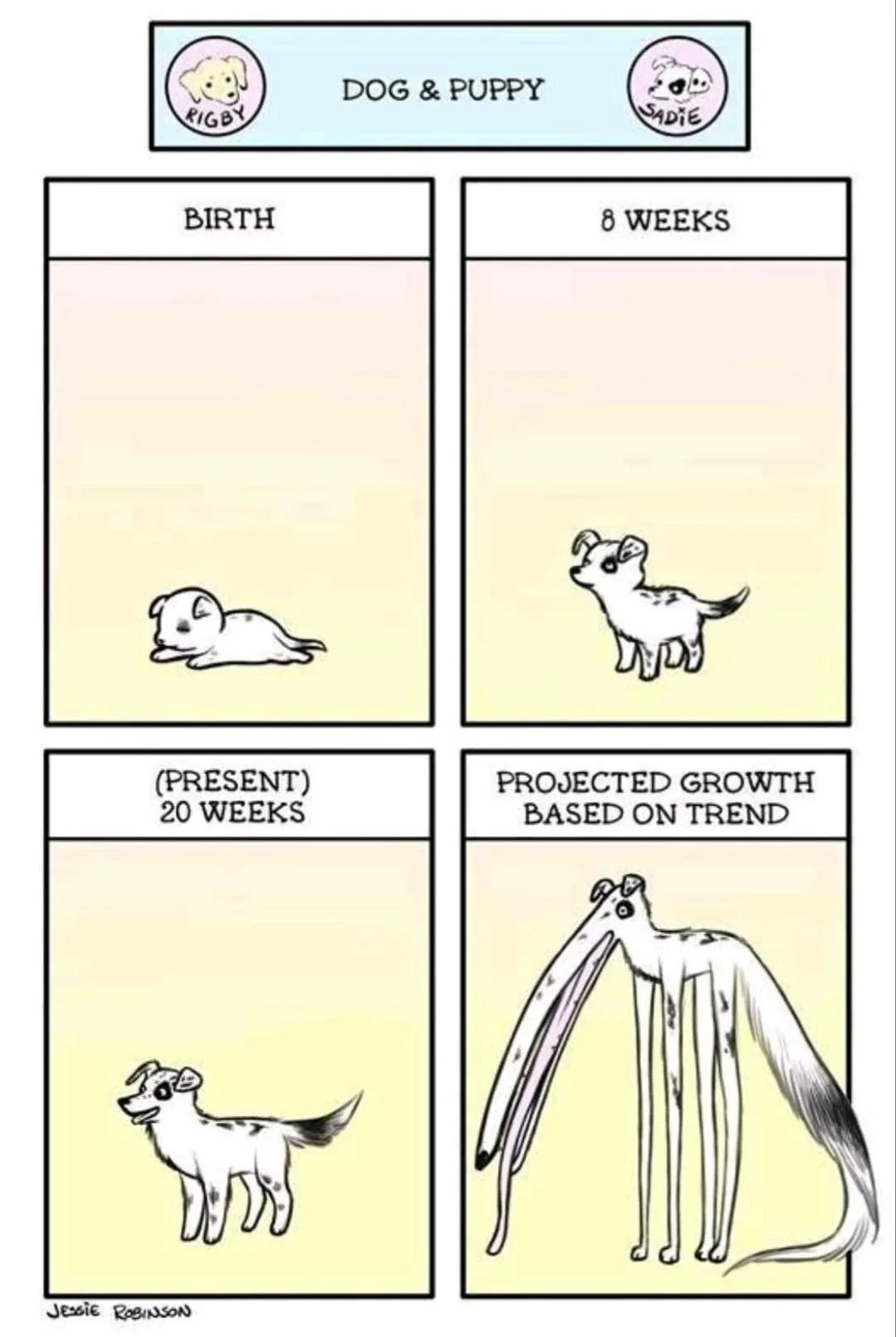
Source: Reddit (original source unclear…)

Code for AR(1) model

function ar1_loglik_whitened(θ, dat)
    # might need to include mean or trend parameters as well
    # subtract trend from data to make this mean-zero in this case
    ρ, σ = θ
    T = length(dat)
    ll = 0 # initialize log-likelihood counter
    for i = 1:T
        if i == 1
            ll += logpdf(Normal(0, sqrt(σ^2 / (1 - ρ^2))), dat[i])
        else
            ll += logpdf(Normal(ρ * dat[i-1], σ), dat[i])
        end
    end
    return ll
end

function ar1_loglik_joint(θ, dat)
    # might need to include mean or trend parameters as well
    # subtract trend from data to make this mean-zero in this case
    ρ, σ = θ
    T = length(dat)
    # compute all of the pairwise lags
    # this is an "outer product"; syntax will differ wildly by language
    H = abs.((1:T) .- (1:T)')
    P = ρ.^H # exponentiate ρ by each lag
    Σ = σ^2 / (1 - ρ^2) * P
    ll = logpdf(MvNormal(zeros(T), Σ), dat)
    return ll
end

ar1_loglik_joint (generic function with 1 method)

AR(1) Example

Code

ρ = 0.6
σ = 0.25
T = 25
ts_sim = zeros(T)
# simulate synthetic AR(1) series
for t = 1:T
    if t == 1
        ts_sim[t] = rand(Normal(0, sqrt(σ^2 / (1 - ρ^2))))
    else
        ts_sim[t] = rand(Normal(ρ * ts_sim[t-1], σ))
    end
end

plot(1:T, ts_sim, linewidth=3, xlabel="Time", ylabel="Value", title=L"$ρ = 0.6, σ = 0.25$")
plot!(size=(600, 500))

Figure 8: Simulated AR(1) data

Code

lb = [-0.99, 0.01]
ub = [0.99, 5]
init = [0.6, 0.3]

optim_whitened = Optim.optimize(θ -> -ar1_loglik_whitened(θ, ts_sim), lb, ub, init)
θ_wn_mle = round.(optim_whitened.minimizer; digits=2)
@show θ_wn_mle;

optim_joint = Optim.optimize(θ -> -ar1_loglik_joint(θ, ts_sim), lb, ub, init)
θ_joint_mle = round.(optim_joint.minimizer; digits=2)
@show θ_joint_mle;

θ_wn_mle = [0.4, 0.2]
θ_joint_mle = [0.4, 0.2]

Key Points

Time series exhibit serial dependence (autocorrelation
AR(1) probability models: joint vs. whitened likelihoods
In general, AR models useful for forecasting/when we don’t care about explanation, pretty useless for explanation.
Similar concepts in spatial data: spatial correlation (distance/adjacency vs. time), lots of different models.

For More On Time Series

Courses

STSCI 4550/5550 (Applied Time Series Analysis),
CEE 6790 (heavy focus on spectral analysis and signal processing)

Books

Shumway & Stoffer (2025)
Hyndman & Athanasopoulos (2021)
Durbin & Koopman (2012)
Banerjee et al. (2011)
Cressie & Wikle (2011)

Discussion of Lloyd & Oreskes (2018)

Questions to Seed Discussion

What was your key takeaway?
What do you think the pros/cons are of the risk and storyline approaches?
How well do you think the authors argued their case?

Upcoming Schedule

Assessments

HW1: Due Friday at 9pm.

Quiz: Available after class.

References

References (Scroll For Full List)

Banerjee, S., Carlin, B. P., & Gelfand, A. E. (2011). Hierarchical modeling and analysis for spatial data, second edition (2nd ed.). Philadelphia, PA: Chapman & Hall/CRC. https://doi.org/10.1201/b17115

Cressie, N., & Wikle, C. K. (2011). Statistics for Spatio-Temporal Data. Hoboken, NJ: Wiley.

Durbin, J., & Koopman, S. J. (2012). Time series analysis by state space methods (2nd ed.). London, England: Oxford University Press. https://doi.org/10.1093/acprof:oso/9780199641178.001.0001

Hyndman, R. J., & Athanasopoulos, G. (2021). Forecasting: Principles and Practice (3rd ed). Melbourne, Australia: OTexts. Retrieved from https://otexts.com/fpp3/

Shumway, R. H., & Stoffer, D. S. (2025). Time series analysis and its applications. Springer.