Uncertainty Quantification and The Bootstrap

Lecture 12

March 5, 2024

Review

Monte Carlo Simulation

Monte Carlo Principle: Approximate \[\mathbb{E}_f[h(X)] = \int h(x) f(x) dx \approx \frac{1}{n} \sum_{i=1}^n h(X_i)\]
Monte Carlo is an unbiased estimator, but beware (and always report) the standard error \(\sigma_n = \sigma_Y / \sqrt{n}\) or confidence intervals.
More advanced methods can reduce variance, but may be difficult to implement in practice.

Uses of Monte Carlo

Estimate expectations / quantiles;
Calculate deterministic quantities (framed as stochastic expectations);
Optimization (problem 3 on HW3).

Sampling Distributions

So Far…

We’re 7 weeks in and haven’t said anything about how to quantify uncertainties.

Let’s talk about that.

Sampling Distributions

The sampling distribution of a statistic captures the uncertainty associated with random samples.

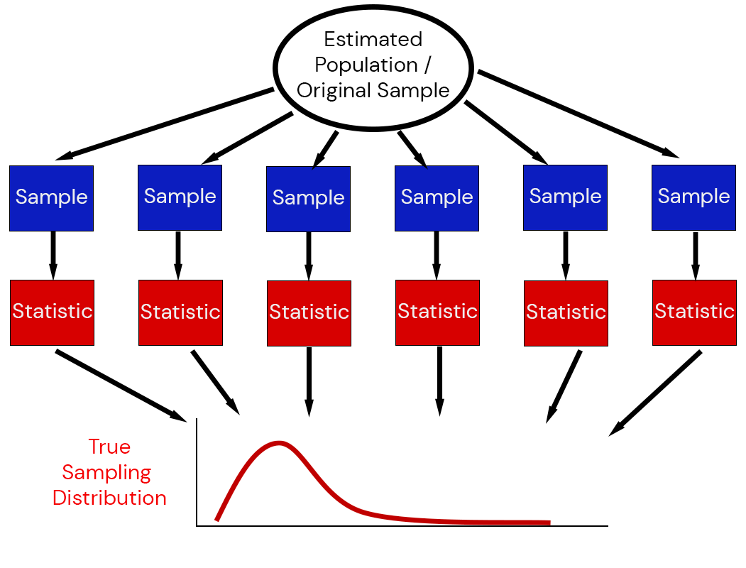
Estimating Sampling Distributions

Special Cases: can derive closed-form representations of sampling distributions (think statistical tests)
Asymptotics: Central Limit Theorem or Fisher Information

Fisher Information

Fisher Information: \[\mathcal{I}_x(\theta) = -\mathbb{E}\left[\frac{\partial^2}{\partial \theta_i \partial \theta_j} \log \mathcal{L}(\theta | x)\right]\]

Observed Fisher Information (uses observed data and calculated at the MLE): \[\mathcal{I}_\tilde{x}(\hat{\theta})\]

Figure 1: Examples of Fisher Information

Fisher Information and Standard Errors

Asymptotic result: \[\sqrt{n}(\theta_\text{MLE} - \theta^*) \to N(0, \left(\mathcal{I}_x(\hat{\theta^*})\right)^{-1}\]

Sampling distribution based on observed data: \[\theta \sim N\left(\hat{\theta}_\text{MLE}, \left(n\mathcal{I}_\tilde{x}(\theta_\text{MLE})\right)^{-1}\right)\]

Estimating Fisher Information

Can be done with automatic differentiation or (sometimes hard) calculations;
May be singular (no inverse ; undefined standard errors) for complex models;
May not be a good approximation of the variance for finite samples!

The Bootstrap

The Bootstrap Principle

Efron (1979) suggested combining estimation with simulation: the bootstrap.

Key idea: use the data to simulate a data-generating mechanism.

Bootstrap Principle

Assume the existing data is representative of the “true” population,
Simulate based on properties of the data itself
Re-estimate statistics from re-samples.

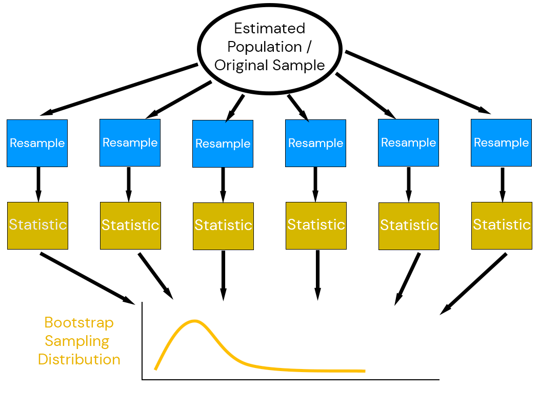
Why Does The Bootstrap Work?

Efron’s key insight: due to the Central Limit Theorem, the bootstrap distribution \(\mathcal{D}(\tilde{t}_i)\) has the same relationship to the observed estimate \(\hat{t}\) as the sampling distribution \(\mathcal{D}(\hat{t})\) has to the “true” value \(t_0\):

\[\mathcal{D}(\tilde{t} - \hat{t}) \approx \mathcal{D}(\hat{t} - t_0)\]

where \(t_0\) the “true” value of a statistic, \(\hat{t}\) the sample estimate, and \((\tilde{t}_i)\) the bootstrap estimates.

What Can We Do With The Bootstrap?

Let \(t_0\) the “true” value of a statistic, \(\hat{t}\) the estimate of the statistic from the sample, and \((\tilde{t}_i)\) the bootstrap estimates.

Estimate Variance: \(\text{Var}[\hat{t}] \approx \text{Var}[\tilde{t}]\)
Bias Correction: \(\mathbb{E}[\hat{t}] - t_0 \approx \mathbb{E}[\tilde{t}] - \hat{t}\)

Notice that bias correction “shifts” away from the bootstrapped samples.

“Simple” Bootstrap Confidence Intervals

Basic Bootstrap CIs (based on CLT for error distribution \(\tilde{t} - \hat{t}\)): \[\left(\hat{t} - (Q_{\tilde{t}}(1-\alpha/2) - \hat{t}), \hat{t} - (Q_{\tilde{t}}(\alpha/2) - \hat{t})\right)\]
Percentile Bootstrap CIs (simplest, often wrong coverage): \[(Q_{\tilde{t}}(1-\alpha/2), Q_{\tilde{t}}(1-\alpha/2))\]

The Non-Parametric Bootstrap

The non-parametric bootstrap is the most “naive” approach to the bootstrap: resample-then-estimate.

Sources of Non-Parametric Bootstrap Error

Sampling error: error from using finitely many replications
Statistical error: error in the bootstrap sampling distribution approximation

Simple Example: Is A Coin Fair?

Suppose we have observed twenty flips with a coin, and want to know if it is weighted.

Code

# define coin-flip model
p_true = 0.6
n_flips = 20
coin_dist = Bernoulli(p_true)
# generate data set
dat = rand(coin_dist, n_flips)
freq_dat = sum(dat) / length(dat)
dat'

1×20 adjoint(::Vector{Bool}) with eltype Bool:
 1  1  0  0  0  1  0  0  0  1  1  1  1  1  1  0  1  1  1  1

The frequency of heads is 0.65.

Is The Coin Fair?

Code

# bootstrap: draw new samples
function coin_boot_sample(dat)
    boot_sample = sample(dat, length(dat); replace=true)
    return boot_sample
end

function coin_boot_freq(dat, nsamp)
    boot_freq = [sum(coin_boot_sample(dat)) for _ in 1:nsamp]
    return boot_freq / length(dat)
end

boot_out = coin_boot_freq(dat, 1000)
q_boot = 2 * freq_dat .- quantile(boot_out, [0.975, 0.025])

p = histogram(boot_out, xlabel="Heads Frequency", ylabel="Count", title="1000 Bootstrap Samples", label=false, right_margin=5mm)
vline!(p, [p_true], linewidth=3, color=:orange, linestyle=:dash, label="True Probability")
vline!(p, [mean(boot_out) ], linewidth=3, color=:red, linestyle=:dash, label="Bootstrap Mean")
vline!(p, [freq_dat], linewidth=3, color=:purple, linestyle=:dot, label="Observed Frequency")
vspan!(p, q_boot, linecolor=:grey, fillcolor=:grey, alpha=0.3, fillalpha=0.3, label="95% CI")
plot!(p, size=(1000, 450))

Figure 2: Bootstrap heads frequencies for 20 resamples.

Larger Sample Example

Code

n_flips = 50
dat = rand(coin_dist, n_flips)
freq_dat = sum(dat) / length(dat)

boot_out = coin_boot_freq(dat, 1000)
q_boot = 2 * freq_dat .- quantile(boot_out, [0.975, 0.025])

p = histogram(boot_out, xlabel="Heads Frequency", ylabel="Count", title="1000 Bootstrap Samples", titlefontsize=20, guidefontsize=18, tickfontsize=16, legendfontsize=16, label=false, bottom_margin=7mm, left_margin=5mm, right_margin=5mm)
vline!(p, [p_true], linewidth=3, color=:orange, linestyle=:dash, label="True Probability")
vline!(p, [mean(boot_out) ], linewidth=3, color=:red, linestyle=:dash, label="Bootstrap Mean")
vline!(p, [freq_dat], linewidth=3, color=:purple, linestyle=:dot, label="Observed Frequency")
vspan!(p, q_boot, linecolor=:grey, fillcolor=:grey, alpha=0.3, fillalpha=0.3, label="95% CI")
plot!(p, size=(1000, 450))

Figure 3: Bootstrap heads frequencies for 1000 resamples.

Why Use The Non-Parametric Bootstrap?

Do not need to rely on variance asymptotics;
Can obtain non-symmetric CIs.
Embarrassingly parallel to simulate new replicates and generate statistics.

When Can’t You Use The Non-Parametric Bootstrap

Maxima/minima
Very extreme values.

Generally, anything very sensitive to outliers which might not be re-sampled.

Bootstrapping with Structured Data

The naive non-parametric bootstrap that we just saw doesn’t work if data has structure, e.g. spatial or temporal dependence.

Simple Bootstrapping Fails with Structured Data

Code

tide_dat = CSV.read(joinpath("data", "surge", "norfolk-hourly-surge-2015.csv"), DataFrame)
surge_resids = tide_dat[:, 5] - tide_dat[:, 3]

p1 = plot(surge_resids, xlabel="Hour", ylabel="(m)", title="Tide Gauge Residuals", label=:false, linewidth=3)
plot!(p1, size=(600, 450))

resample_index = sample(1:length(surge_resids), length(surge_resids); replace=true)
p2 = plot(surge_resids[resample_index], xlabel="Hour", ylabel="(m)", title="Tide Gauge Resample", label=:false, linewidth=3)
plot!(p2, size=(600, 450))

display(p1)
display(p2)

(a) Simple bootstrap with time series data.

(b)

Figure 4

Block Bootstraps

Clever idea from Kunsch (1989): Divide time series \(y_{1:T}\) into overlapping blocks of length \(k\).

\[\{y_{1:k}, y_{2:k+1}, \ldots y_{n-k+1:n}\}\]

Then draw \(m = n / k\) of these blocks with replacement and construct replicate time series:

\[\hat{y}_{1:n} = (y_{b_1}, \ldots, y_{b_m}) \]

Note: Your series must not have a trend!

Block Bootstrap Example

Code

k = 20
n_blocks = length(surge_resids) - k + 1
blocks = zeros(Float64, (k, n_blocks))
for i = 1:n_blocks
    blocks[:, i] = surge_resids[i:(k+i-1)]
end
blocks[:, 1:5]

20×5 Matrix{Float64}:
  0.136   0.107   0.097   0.093   0.093
  0.107   0.097   0.093   0.093   0.08
  0.097   0.093   0.093   0.08    0.068
  0.093   0.093   0.08    0.068   0.031
  0.093   0.08    0.068   0.031   0.005
  0.08    0.068   0.031   0.005   0.011
  0.068   0.031   0.005   0.011   0.012
  0.031   0.005   0.011   0.012   0.001
  0.005   0.011   0.012   0.001  -0.002
  0.011   0.012   0.001  -0.002  -0.014
  0.012   0.001  -0.002  -0.014  -0.013
  0.001  -0.002  -0.014  -0.013  -0.015
 -0.002  -0.014  -0.013  -0.015  -0.02
 -0.014  -0.013  -0.015  -0.02   -0.019
 -0.013  -0.015  -0.02   -0.019  -0.031
 -0.015  -0.02   -0.019  -0.031  -0.071
 -0.02   -0.019  -0.031  -0.071  -0.067
 -0.019  -0.031  -0.071  -0.067  -0.084
 -0.031  -0.071  -0.067  -0.084  -0.086
 -0.071  -0.067  -0.084  -0.086  -0.092

Code

m = Int64(ceil(length(surge_resids) / k))
n_boot = 1_000
surge_bootstrap = zeros(length(surge_resids), n_boot)
for i = 1:n_boot
    block_sample_idx = sample(1:n_blocks, m; replace=true)
    surge_bootstrap[:, i] = reduce(vcat, blocks[:, block_sample_idx])
end

p = plot(surge_resids, color=:black, lw=3, label="Data", xlabel="Hour", ylabel="(m)", title="Tide Gauge Residuals", alpha=0.5)
plot!(p, surge_bootstrap[:, 1], color=:blue, lw=3, label="Replicate", alpha=0.5)
plot!(p, size=(600, 500))

Figure 5: Comparison of original data with block bootstrap replicate.

Block Bootstrap Replicates

Code

p = plot(xlabel="Hour", ylabel="(m)", title="Tide Gauge Residuals")
for i = 1:10
    label = i == 1 ? "Replicate" : false
    plot!(p, surge_bootstrap[:, i], label=label, color=:gray, alpha=0.2, lw=2)
end
plot!(p, surge_resids, label="Data", color=:black, lw=3)
plot!(p, size=(1200, 500))

Figure 6: Block bootstrap with time series data.

Generalizing the Block Bootstrap

Circular Bootstrap: “Wrap” the time series in a circle, \(y_1, y_2, \ldots, y_n, y_1, y_2, \ldots\) then divide into blocks and resample.
Stationary Bootstrap: Use random block lengths to avoid systematic boundary transitions.
Block of Blocks Bootstrap: Divide series into blocks of length \(k_2\), then subdivide into blocks of length \(k_1\). Sample blocks with replacement then sample sub-blocks within each block with replacement.

Key Points and Upcoming Schedule

Key Points

Bootstrap: Approximate sampling distribution by re-simulating data
Non-Parametric Bootstrap: Treat data as representative of population and re-sample.
More complicated for structured data: block bootstrap for time series, analogues for spatial data.

Sources of Non-Parametric Bootstrap Error

Sampling error: error from using finitely many replications
Statistical error: error in the bootstrap sampling distribution approximation

When To Use The Non-Parametric Bootstrap

Sample is representative of the sampling distribution
Doesn’t work well for extreme values!
Does not work at all for max/mins (or any other case where the CLT fails).

Next Classes

Monday: The Parametric Bootstrap

Wednesday: What is a Markov Chain?

Assessments

Homework 3: Due next Friday (3/14)

Project Proposals: Due 3/21.

References

References (Scroll for Full List)

Efron, B. (1979). Bootstrap methods: Another look at the jackknife. Ann. Stat., 7, 1–26. https://doi.org/10.1214/aos/1176344552

Kunsch, H. R. (1989). The jackknife and the bootstrap for general stationary observations. Ann. Stat., 17, 1217–1241. https://doi.org/10.1214/aos/1176347265