Then the bootstrap error distribution approximates the sampling distribution \[(\tilde{t}_i - \hat{t}) \overset{\mathcal{D}}{\sim} \hat{t} - t_0\]
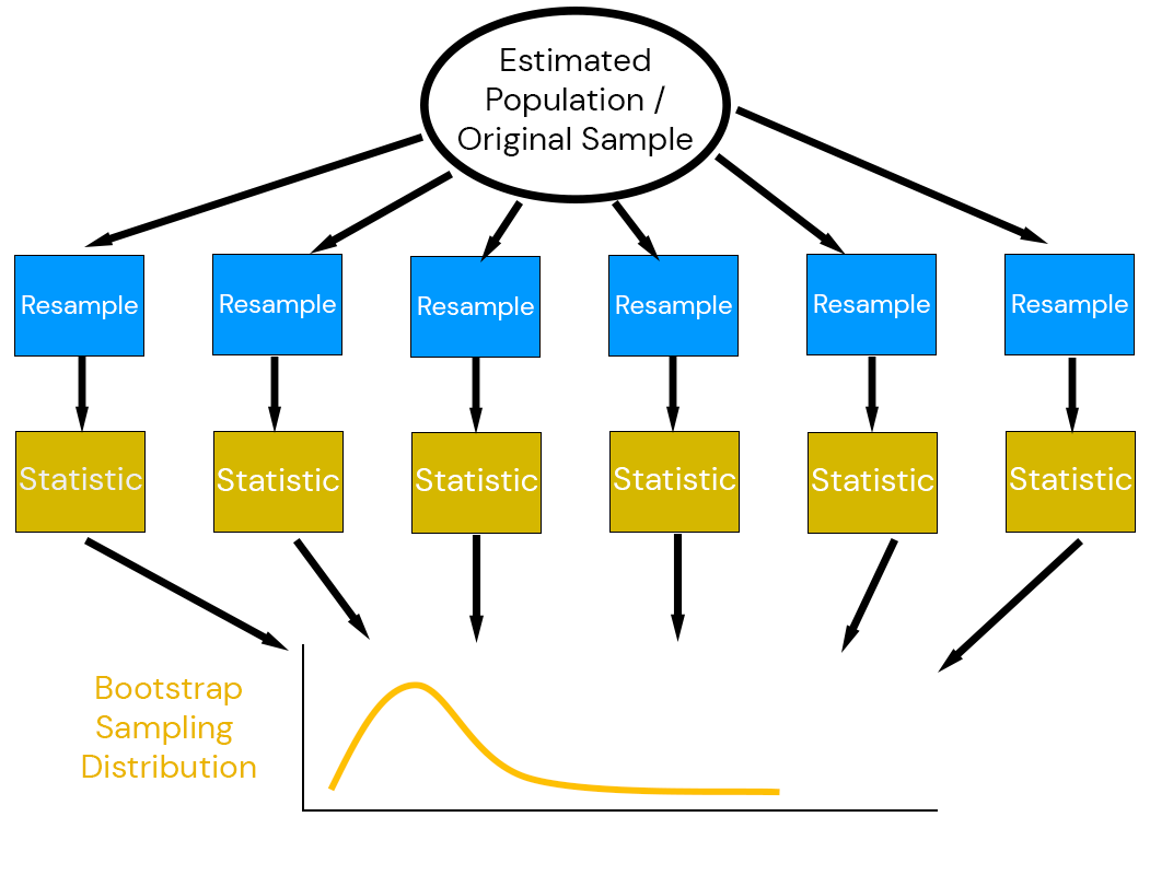
The Non-Parametric Bootstrap
The non-parametric bootstrap is the most “naive” approach to the bootstrap: resample-then-estimate.
Non-Parametric Bootstrap
Approaches to Bootstrapping Structured Data
Correlations: Transform to uncorrelated data (principal components, etc.), sample, transform back.
Time Series: Block bootstrap
Sources of Non-Parametric Bootstrap Error
Sampling error: error from using finitely many replications
Statistical error: error in the bootstrap sampling distribution approximation
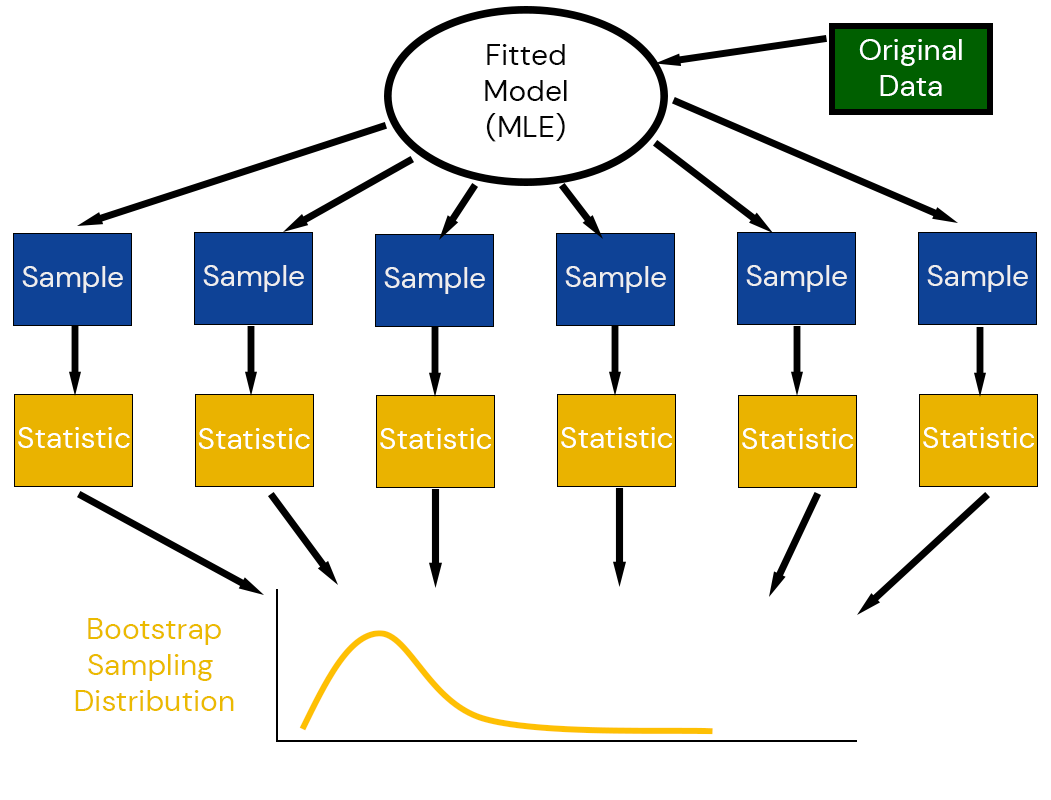
The Parametric Bootstrap
The Parametric Bootstrap
Non-Parametric Bootstrap: Resample directly from the data.
Parametric Bootstrap: Fit a model to the original data and simulate new samples, then calculate bootstrap estimates.
This lets us use additional information, such as a simulation or statistical model, instead of relying only on the empirical CDF.
Parametric Bootstrap Scheme
The parametric bootstrap generates pseudodata using simulations from a fitted model.
Parametric Bootstrap
Benefits of the Parametric Bootstrap
Can quantify uncertainties in parameter values
Deals better with structured data (model accounts for structure)
Can look at statistics which are limited by resimulating from empirical CDF.
Potential Drawbacks
New source of error: model specification
Misspecified models can completely distort estimates.
Example: 100-Year Return Periods
Tide Gauge Data
Detrended San Francisco Tide Gauge Data:
Code
# read in data and get annual maximafunctionload_data(fname) date_format =DateFormat("yyyy-mm-dd HH:MM:SS")# This uses the DataFramesMeta.jl package, which makes it easy to string together commands to load and process data df =@chain fname begin CSV.read(DataFrame; header=false)rename("Column1"=>"year", "Column2"=>"month", "Column3"=>"day", "Column4"=>"hour", "Column5"=>"gauge")# need to reformat the decimal date in the data file@transform:datetime =DateTime.(:year, :month, :day, :hour)# replace -99999 with missing@transform:gauge =ifelse.(abs.(:gauge) .>=9999, missing, :gauge)select(:datetime, :gauge)endreturn dfenddat =load_data("data/surge/h551.csv")# detrend the data to remove the effects of sea-level rise and seasonal dynamicsma_length =366ma_offset =Int(floor(ma_length/2))moving_average(series,n) = [mean(@view series[i-n:i+n]) for i in n+1:length(series)-n]dat_ma =DataFrame(datetime=dat.datetime[ma_offset+1:end-ma_offset], residual=dat.gauge[ma_offset+1:end-ma_offset] .-moving_average(dat.gauge, ma_offset))# group data by year and compute the annual maximadat_ma =dropmissing(dat_ma) # drop missing datadat_annmax =combine(dat_ma -> dat_ma[argmax(dat_ma.residual), :], groupby(transform(dat_ma, :datetime =>x->year.(x)), :datetime_function))delete!(dat_annmax, nrow(dat_annmax)) # delete 2023; haven't seen much of that year yetrename!(dat_annmax, :datetime_function =>:Year)select!(dat_annmax, [:Year, :residual])dat_annmax.residual = dat_annmax.residual /1000# convert to m# make plotsp1 =plot( dat_annmax.Year, dat_annmax.residual; xlabel="Year", ylabel="Annual Max Tide (m)", label=false, marker=:circle, markersize=5)p2 =histogram( dat_annmax.residual, normalize=:pdf, orientation=:horizontal, label=:false, xlabel="PDF", ylabel="", yticks=[])l =@layout [a{0.7w} b{0.3w}]plot(p1, p2; layout=l, link=:y, ylims=(1, 1.7), bottom_margin=10mm, left_margin=5mm)plot!(size=(1000, 400))
Figure 1: Annual maxima surge data from the San Francisco, CA tide gauge.
Parametric Bootstrap Strategy
Fit/calibrate model
Compute statistic of interest
Repeat \(N\) times:
Resample values from fitted model
Calculate statistic.
Compute mean/confidence intervals from distribution of bootstrapped statistics.
Parametric Bootstrap Results
Code
# function to fit GEV model for each data setinit_θ = [1.0, 1.0, 0.0]lb = [0.0, 0.0, -2.0]ub = [5.0, 10.0, 2.0]loglik_gev(θ) =-sum(logpdf(GeneralizedExtremeValue(θ[1], θ[2], θ[3]), dat_annmax.residual))# get estimates from observationsrp_emp =quantile(dat_annmax.residual, 0.99)θ_gev = Optim.optimize(loglik_gev, lb, ub, init_θ).minimizerp =histogram(dat_annmax.residual, normalize=:pdf, xlabel="Annual Maximum Storm Tide (m)", ylabel="Probability Density", label=false, right_margin=5mm)plot!(p, GeneralizedExtremeValue(θ_gev[1], θ_gev[2], θ_gev[3]), linewidth=3, label="Parametric Model", color=:orange)vline!(p, [rp_emp], color=:red, linewidth=3, linestyle=:dash, label="Empirical Return Level")vline!(p, [quantile(GeneralizedExtremeValue(θ_gev[1], θ_gev[2], θ_gev[3]), 0.99)], color=:blue, linewidth=3, linestyle=:dash, label="Model Return Level")xlims!(p, 1, 2)
Parametric bootstrap estimates converge faster than non-parametric estimates.
If your parametric model is “properly” specified, parametric bootstrap gives more accurate results with the same \(n\).
If the parametric model is mis-specified, you’re rapidly converging to the wrong distribution.
Bootstrapping Residuals
Can bootrap residuals from a model versus “full” parametric bootstrap:
Fit model (statistically or numerical).
Calculate residuals from deterministic/expected values.
Resample residuals.
Add bootstrapped residuals back to model trend to create new replicates.
Refit model to replicates.
Last Thoughts on the Bootstrap
Bootstrap vs. Monte Carlo
Bootstrap “if I had a different sample (conditional on the bootstrap principle), what could I have inferred”?
Monte Carlo: Given specification of input uncertainty, what data could we generate?
Bootstrap Distribution and Monte Carlo
Could we use a bootstrap distribution for MC?
Sure, that’s just one specification of the data-generating process.
Nothing unique or particularly rigorous in using the bootstrap for this; substituting the bootstrap principle for other assumptions.
Bootstrap vs. Bayes
Bootstrap: “if I had a different sample (conditional on the bootstrap principle), what could I have inferred”?
Bayesian Inference: “what different parameters could have produced the observed data”?
Key Points
Key Points
Bootstrap: Use the characteristics of the data to simulate new samples.
Bootstrap gives idea of sampling error in statistics (including model parameters)
Distribution of \(\tilde{t} - \hat{t}\) approximates distribution around estimate \(\hat{t} - t_0\).
Allows us to estimate uncertainty of estimates (confidence intervals, bias, etc).
Parametric bootstrap introduces model specification error
Bootstrap Variants
Resample Cases (Non-Parametric)
Resample Residuals (from fitted model trend)
Simulate from Fitted Model (Parametric)
Which Bootstrap To Use?
Depends on trust in model “correctness”: - Do we trust the model specification to be reasonably correct? - Do we trust that we have enough samples to recover the empirical CDF? - Do we trust the data-generating process?
Discussion of Bankes et al (1993)
Questions to Seed Discussion
What are the practical differences between exploratory and consolidative modeling?
When do you think each approach is more or less appropriate?
How do these approaches impact the choice of your methods?