Bayesian Computing and MCMC
Lecture 14
March 12, 2024
Last Classes
The Bootstrap

Why Does The Bootstrap Work?
Let \(t_0\) the “true” value of a statistic, \(\hat{t}\) the estimate of the statistic from the sample, and \((\tilde{t}_i)\) the bootstrap estimates.
- Variance: \(\text{Var}[\hat{t}] \approx \text{Var}[\tilde{t}]\)
- Then the bootstrap error distribution approximates the sampling distribution \[(\tilde{t}_i - \hat{t}) \overset{\mathcal{D}}{\sim} \hat{t} - t_0\]
Bootstrap Variants
- Resample Cases (Non-Parametric)
- Resample Residuals (from fitted model trend)
- Simulate from Fitted Model (Parametric)
Which Bootstrap To Use?
Depends on trust in model “correctness”: - Do we trust the model specification to be reasonably correct? - Do we trust that we have enough samples to recover the empirical CDF? - Do we trust the data-generating process?
Bayesian Computing
Sampling So Far
Rejection sampling (or importance sampling) to draw i.i.d. samples from a proposal density and reject/re-weight based on target.
Both require \(f(x) \leq M g(x)\) for some \(1 < M < \infty\).
Bayesian Computing Challenges
- Samples needed to compute posterior quantities (credible intervals, posterior predictive distributions, model skill estimates, etc.) with Monte Carlo.
- Posteriors often highly correlated.
- Grid approximation can help us visualize the posteriors in low dimensions.
- Rejection sampling scales poorly to higher dimensions.
- Conjugate priors only are appropriate in limited cases.
What Would Make A Good Algorithm?
A wishlist:
- Don’t need to know the characteristics of the distribution.
- Samples will eventually be correctly distributed (given enough time).
- Ideally fast and requiring minimal tuning.
How Can We Do This?
Suppose we want to sample a probability distribution \(f(\cdot)\) and are at a parameter vector \(x\).
What if we had a method that would let us stochastically jump from \(x\) to a new vector \(y\) in such a way that, eventually, we would visit any given vector wiith probability \(f\)?
This would let us trade convenience/flexibility for dependent samples.
Markov Chain Monte Carlo (MCMC)
There is a mathematical process that has these properties: Markov Chains.
These methods are called Markov chain Monte Carlo (MCMC).
Markov Chains
What Is A Markov Chain?
Consider a stochastic process \(\{X_t\}_{t \in \mathcal{T}}\), where
- \(X_t \in \mathcal{S}\) is the state at time \(t\), and
- \(\mathcal{T}\) is a time-index set (can be discrete or continuous)
- \(\mathbb{P}(s_i \to s_j) = p_{ij}\).
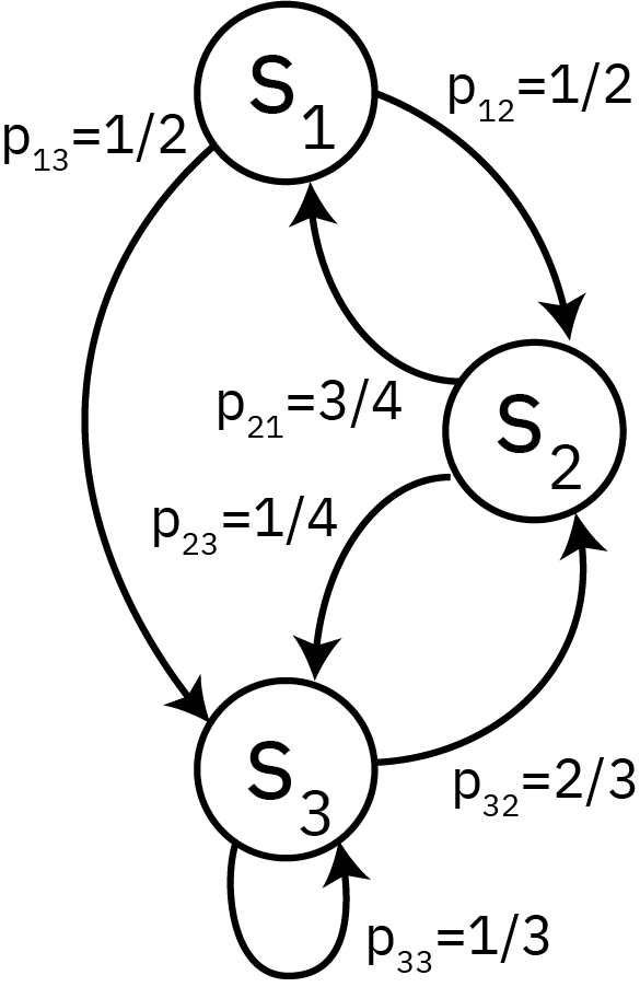
Markovian Property
This stochastic process is a Markov chain if it satisfies the Markovian (or memoryless) property: \[\begin{align*} \mathbb{P}(X_{T+1} = s_i &| X_1=x_1, \ldots, X_T=x_T) = \\ &\qquad\mathbb{P}(X_{T+1} = s_i| X_T=x_T) \end{align*} \]
Example: “Drunkard’s Walk”
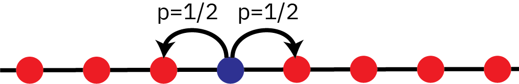
- How can we model the unconditional probability \(\mathbb{P}(X_T = s_i)\)?
- How about the conditional probability \(\mathbb{P}(X_T = s_i | X_{T-1} = x_{T-1})\)?
Example: Weather
Suppose the weather can be foggy, sunny, or rainy.
Based on past experience, we know that:
- There are never two sunny days in a row;
- Even chance of two foggy or two rainy days in a row;
- A sunny day occurs 1/4 of the time after a foggy or rainy day.
Aside: Higher Order Markov Chains
Suppose that today’s weather depends on the prior two days.
- Can we write this as a Markov chain?
- What are the states?
Weather Transition Matrix
We can summarize these probabilities in a transition matrix \(P\): \[ P = \begin{array}{cc} \begin{array}{ccc} \phantom{i}\color{red}{F}\phantom{i} & \phantom{i}\color{red}{S}\phantom{i} & \phantom{i}\color{red}{R}\phantom{i} \end{array} \\ \begin{pmatrix} 1/2 & 1/4 & 1/4 \\ 1/2 & 0 & 1/2 \\ 1/4 & 1/4 & 1/2 \end{pmatrix} & \begin{array}{ccc} \color{red}F \\ \color{red}S \\ \color{red}R \end{array} \end{array} \]
Rows are the current state, columns are the next step, so \(\sum_i p_{ij} = 1\).
Weather Example: State Probabilities
Denote by \(\lambda^t\) a probability distribution over the states at time \(t\).
Then \(\lambda^t = \lambda^{t-1}P\):
\[\begin{pmatrix}\lambda^t_F & \lambda^t_S & \lambda^t_R \end{pmatrix} = \begin{pmatrix}\lambda^{t-1}_F & \lambda^{t-1}_S & \lambda^{t-1}_R \end{pmatrix} \begin{pmatrix} 1/2 & 1/4 & 1/4 \\ 1/2 & 0 & 1/2 \\ 1/4 & 1/4 & 1/2 \end{pmatrix} \]
Multi-Transition Probabilities
Notice that \[\lambda^{t+i} = \lambda^t P^i,\] so multiple transition probabilities are \(P\)-exponentials.
\[P^3 = \begin{array}{cc} \begin{array}{ccc} \phantom{iii}\color{red}{F}\phantom{ii} & \phantom{iii}\color{red}{S}\phantom{iii} & \phantom{ii}\color{red}{R}\phantom{iii} \end{array} \\ \begin{pmatrix} 26/64 & 13/64 & 25/64 \\ 26/64 & 12/64 & 26/64 \\ 26/64 & 13/64 & 26/64 \end{pmatrix} & \begin{array}{ccc} \color{red}F \\ \color{red}S \\ \color{red}R \end{array} \end{array} \]
Long Run Probabilities
What happens if we let the system run for a while starting from an initial sunny day?
Code
current = [1.0, 0.0, 0.0]
P = [1/2 1/4 1/4
    1/2 0 1/2
    1/4 1/4 1/2]

T = 21

state_probs = zeros(T, 3)
state_probs[1,:] = current
for t=1:T-1
    state_probs[t+1, :] = state_probs[t:t, :] * P
end


p = plot(0:T-1, state_probs, label=["Foggy" "Sunny" "Rainy"], palette=:mk_8, linewidth=3)
xlabel!("Time")
ylabel!("State Probability")
plot!(p, size=(1000, 350))Stationary Distributions
This stabilization always occurs when the probability distribution is an eigenvector of \(P\) with eigenvalue 1:
\[\pi = \pi P.\]
This is called an invariant or a stationary distribution.
Which Markov Chains Have Stationary Distributions?
This is a property called ergodicity (or the chain is ergodic). Ergodic Markov chains always have a limiting distribution which is the limit of the time-evolution of the chain dynamics, e.g. \[\pi_j = \lim_{t \to \infty} \mathbb{P}(X_t = s_j).\]
Key: The limiting distribution is independent of the initial state probability.
Limiting Distributions are Stationary
For an ergodic chain, the limiting distribution is the unique stationary distribution (we won’t prove uniqueness):
\[ \begin{align} \pi_j &= \lim_{t \to \infty} \mathbb{P}(X_t = s_j | X_0 = s_i) \\ &= \lim_{t \to \infty} (P^{t+1})_{ij} = \lim_{t \to \infty} (P^tP)_{ij} \\ &= \lim_{t \to \infty} \sum_d (P^t)_{id} P_{dj} \\ &= \sum_d \pi_d P_{dj} \end{align} \]
MCMC and Ergodic Chains
Proving that a chain is ergodic is getting into the mathematical weeds a bit (and is outside the scope of this class).
The good news: The goal of any MCMC algorithm is to construct an ergodic chain where the stationary distribution \(\pi(\cdot)\) is the target \(f(\cdot)\).
This means that if you’re using a “standard” algorithm, the existence of a stationary distribution for the produced Markov chain is mathematically guaranteed.
Transient Portion of the Chain
The portion of the chain prior to convergence to the stationary distribution is called the transient portion.
Key Points and Upcoming Schedule
Key Points (Bayesian Computing)
- Bayesian computation is difficult because we need to sample from effectively arbitrary distributions.
- Markov chains provide a path forward if we can construct a chain satisfying detailed balance whose stationary distribution is the target distribution.
- Then a post-convergence chain of samples is the same as a dependent Monte Carlo set of samples.
Key Points (Markov Chains)
- Stochastic process with memoryless property.
- Some chains have a stationary distribution (eigenvector of transition matrix with eigenvalue 1).
- Ergodic Markov chains: dynamics converge to a limiting distribution, which is also stationary.
Next Classes
Monday: MCMC
Wednesday: Cross-Validation and Model Skill
Assessments
- Homework 3: Due Friday (3/14)
- Project Proposal: Due 3/21
References
References (Scroll for Full List)
Efron, B. (1979). Bootstrap methods: Another look at the jackknife. Ann. Stat., 7, 1–26. https://doi.org/10.1214/aos/1176344552