Ergodic chains: dynamics converge to limiting distribution \[\pi_j = \lim_{n \to \infty} \mathbb{P}(X_n = s_j)\] which is stationary, \(\pi = \pi P\).
Markov Chain Monte Carlo
Family of methods for simulating from hard-to-sample from distributions \(\pi\);
Rely on ergodic Markov chains for simulation;
By construction, chains converge to limiting distribution which is the target distribution \(\pi\).
MCMC Overview
Detailed Balance
Let \(\{X_t\}\) be a Markov chain and let \(\pi\) be a probability distribution over the states. Then the chain is in detailed balance with respect to \(\pi\) if \[\pi_i P_{ij} = \pi_j P_{ji}.\]
Detailed balance implies reversibility: the chain’s dynamics are the same when viewed forwards or backwards in time.
The idea of our sampling algorithm is to construct an ergodic Markov chain from the detailed balance equation for the target distribution.
Detailed balance implies that the target distribution is the stationary distribution.
Ergodicity implies that this distribution is unique and can be obtained as the limiting distribution of the chain’s dynamics.
Idea of Sampling Algorithm
In other words:
Generate an appropriate Markov chain so that its stationary distribution of the target distribution \(\pi\);
Run its dynamics long enough to converge to the stationary distribution;
Use the resulting ensemble of states as Monte Carlo samples from \(\pi\) .
Sampling Algorithm
Any algorithm which follows this procedure is a Markov chain Monte Carlo algorithm.
Good news: These algorithms are designed to work quite generally, without (usually) having to worry about technical details like detailed balance and ergodicity.
Bad news: They can involve quite a bit of tuning for computational efficiency. Some algorithms or implementations are faster/adaptive to reduce this need.
Sampling Algorithm
Annoying news:
Convergence to the stationary distribution is only guaranteed asymptotically; evaluating if the chain has been run long enough requires lots of heuristics.
Due to Markovian property, samples are autocorrelated, so smaller “effective sample size” than the raw number of samples.
What Is The Upshot?
Given a Markov chain \(\{X_t\}_{t=1, \ldots, T}\) returned from MCMC, sampling from distribution \(\pi\):
\(\mathbb{P}(X_t = y) \to \pi(y)\) as \(t \to \infty\)
This means the chain can be considered a dependent sample approximately distributed from \(\pi\).
The first values (the transient portion) of the chain are highly dependent on the initial value but do not affect asymptotic convergence.
History of MCMC
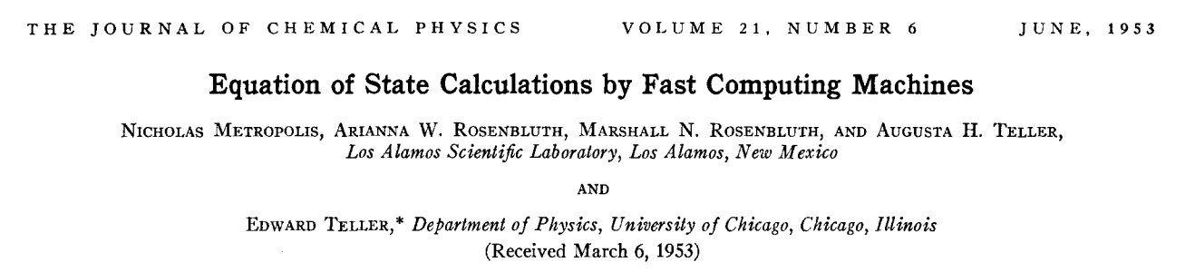
Metropolis et al
“…instead of choosing configurations randomly, then weighting them with \(\exp(- E/ kT)\), we choose configurations with a probability \(\exp (- E/ kT)\) and weight them evenly.”
Example: Metropolis-Hastings
Given \(X_t = x_t\):
Generate \(Y_t \sim q(y | x_t)\);
Set \(X_{t+1} = Y_t\) with probability \(\rho(x_t, Y_t)\), where \[\rho(x, y) = \min \left\{\frac{\pi(y)}{\pi(x)}\frac{q(x | y)}{q(y | x)}, 1\right\},\] else set \(X_{t+1} = x_t\).
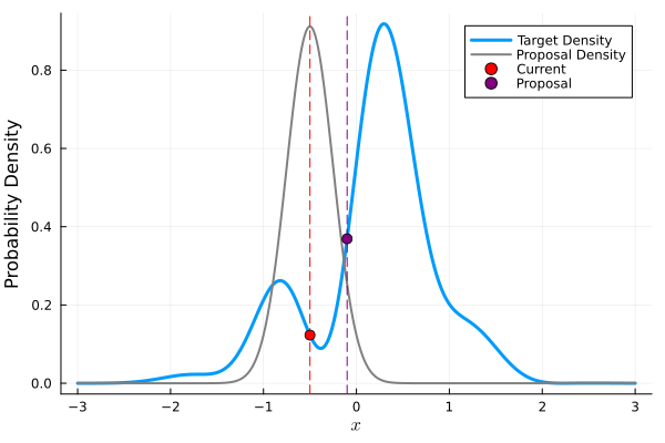
M-H Algorithm Illustration
First Example of M-H Algorithm
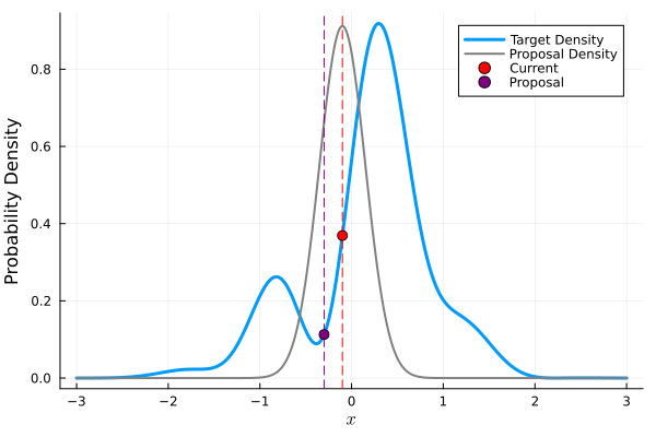
Second Example of M-H Algorithm
How Simple Is That?
The devil is in the details: performance and efficiency are highly dependent on the choice of \(q\).
Key: There is a tradeoff between exploration and acceptance.
Wide proposal: Can make bigger jumps, may be more likely to reject proposals.
Narrow proposal: More likely to accept proposals, may not “mix” efficiently.
More Modern MCMC Algorithms
Many innovations in the last decade: best methods use gradients and don’t require much tuning.
These days, no real reason to not use Hamiltonian Monte Carlo (default in pyMC3, Turing, Stan, other probabilistic programming languages) unless you can’t write your code in a PPL.
Sampling With MCMC Using A PPL
San Francisco Tide Gauge Data
Code
# read in data and get annual maximafunctionload_data(fname) date_format =DateFormat("yyyy-mm-dd HH:MM:SS")# This uses the DataFramesMeta.jl package, which makes it easy to string together commands to load and process data df =@chain fname begin CSV.read(DataFrame; header=false)rename("Column1"=>"year", "Column2"=>"month", "Column3"=>"day", "Column4"=>"hour", "Column5"=>"gauge")# need to reformat the decimal date in the data file@transform:datetime =DateTime.(:year, :month, :day, :hour)# replace -99999 with missing@transform:gauge =ifelse.(abs.(:gauge) .>=9999, missing, :gauge)select(:datetime, :gauge)endreturn dfenddat =load_data("data/surge/h551.csv")# detrend the data to remove the effects of sea-level rise and seasonal dynamicsma_length =366ma_offset =Int(floor(ma_length/2))moving_average(series,n) = [mean(@view series[i-n:i+n]) for i in n+1:length(series)-n]dat_ma =DataFrame(datetime=dat.datetime[ma_offset+1:end-ma_offset], residual=dat.gauge[ma_offset+1:end-ma_offset] .-moving_average(dat.gauge, ma_offset))# group data by year and compute the annual maximadat_ma =dropmissing(dat_ma) # drop missing datadat_annmax =combine(dat_ma -> dat_ma[argmax(dat_ma.residual), :], groupby(DataFrames.transform(dat_ma, :datetime =>x->year.(x)), :datetime_function))delete!(dat_annmax, nrow(dat_annmax)) # delete 2023; haven't seen much of that year yetrename!(dat_annmax, :datetime_function =>:Year)select!(dat_annmax, [:Year, :residual])dat_annmax.residual = dat_annmax.residual /1000# convert to m# make plotsp1 =plot( dat_annmax.Year, dat_annmax.residual; xlabel="Year", ylabel="Annual Max Tide Level (m)", label=false, marker=:circle, markersize=5, tickfontsize=16, guidefontsize=18)p2 =histogram( dat_annmax.residual, normalize=:pdf, orientation=:horizontal, label=:false, xlabel="PDF", ylabel="", yticks=[], tickfontsize=16, guidefontsize=18)l =@layout [a{0.7w} b{0.3w}]plot(p1, p2; layout=l, link=:y, ylims=(1, 1.7), bottom_margin=5mm, left_margin=5mm)plot!(size=(1000, 450))
Figure 1: Annual maxima surge data from the San Francisco, CA tide gauge.
usingTuring## y: observed data## can also specify covariates or auxiliary data in the function if used@modelfunctiontide_model(y)# specify priors μ ~Normal(0, 0.5) σ ~truncated(Normal(0, 0.1), 0, Inf)# specify likelihood y ~LogNormal(μ, σ)# returning y allows us (later) to generate predictive simulationsreturn y end
Sampling from Posterior
Code
m =tide_model(dat_annmax.residual)# draw 10_000 samples using NUTS() sampler, with 4 chains (using MCMCThreads() for serial sampling)surge_chain =sample(m, NUTS(), MCMCThreads(), 10_000, 4, progress=false)
┌ Warning: Only a single thread available: MCMC chains are not sampled in parallel
└ @ AbstractMCMC ~/.julia/packages/AbstractMCMC/kwj9g/src/sample.jl:384┌ Info: Found initial step size
└ ϵ = 0.05
┌ Info: Found initial step size
└ ϵ = 0.05
┌ Info: Found initial step size
└ ϵ = 0.05
┌ Info: Found initial step size
└ ϵ = 0.05
Chains MCMC chain (10000×14×4 Array{Float64, 3}):
Iterations = 1001:1:11000
Number of chains = 4
Samples per chain = 10000
Wall duration = 6.29 seconds
Compute duration = 5.06 seconds
parameters = μ, σ
internals = lp, n_steps, is_accept, acceptance_rate, log_density, hamiltonian_energy, hamiltonian_energy_error, max_hamiltonian_energy_error, tree_depth, numerical_error, step_size, nom_step_size
Use `describe(chains)` for summary statistics and quantiles.
What Does This Output Mean?
MCSE: Monte Carlo Standard Error for mean.
ESS (Effective Sample Size): Accounts for autocorrelation \(\rho_t\) across samples \[N_\text{eff} = \frac{N}{1+2\sum_{t=1}^\infty \rho_t}\]
Rhat: Convergence metric (Gelman & Rubin (1992)) based on multiple chains.
Visualizing the Sampler
Code
plot(surge_chain, size=(1200, 500))
Figure 2: Posterior samples from Turing.jl
Assessing Convergence
What Can Go Wrong?
MCMC Sampling for Various Proposals
Autocorrelation of Chains
MCMC Sampling for Various Proposals
How To Identify Convergence?
Short answer: There is no guarantee! Judgement based on an accumulation of evidence from various heuristics.
The good news — getting the precise “right” end of the transient chain doesn’t matter.
If a few transient iterations remain, the effect will be washed out with a large enough post-convergence chain.
Heuristics for Convergence
Compare distribution (histogram/kernel density plot) after half of the chain to full chain.
Run multiple chains from “overdispersed” starting points
Compare intra-chain and inter-chain variances
Summarized as \(\hat{R}\) statistic: closer to 1 implies better convergence.
On Multiple Chains
Unless a specific parallelized scheme (called sequential Monte Carlo) is used, cannot run multiple shorter chains in lieu of one longer chain since each chain needs to individually converge.
This means multiple chains are more useful for diagnostics. But you can sample from each once they’ve converged.
Heuristics for Convergence
If you’re more interested in the mean estimate, can also look at the its stability by iteration or the Monte Carlo standard error.
Look at traceplots; do you see sudden “jumps”?
When in doubt, run the chain longer.
Transient Chain Portion
What do we do with the transient portion of the chain?
Discard as burn-in (might be done automatically by a PPL);
Just run the chain longer.
What To Do After?
Can compute expectations using the full chain; MCSE is more complicated but is reported from most PPL outputs (otherwise platform specific implementations).
Can subsample from or thin chain if computationally convenient (but pay attention to \(ESS\)).
Must rely on “accumulation of evidence” from heuristics for determination about convergence to stationary distribution.
Transient portion of chain: Meh. Some people worry about this too much. Discard or run the chain longer.
Parallelizing solves few problems, but running multiple chains can be useful for diagnostics.
Next Classes
Wednesday: Cross-Validation and Model Skill
Next Week: Entropy and Information Criteria
Assessments
Homework 3: Due Friday (3/14)
Project Proposal: Due 3/21
References
References (Scroll for Full List)
Gelman, A., & Rubin, D. B. (1992). Inference from Iterative Simulation Using Multiple Simulations. Stat. Sci., 7, 457–511. https://doi.org/10.1214/ss/1177011136