Predictive Model Assessments
Lecture 16
March 19, 2024
Last Class
Markov Chain Monte Carlo
- Family of methods for simulating from hard-to-sample from distributions \(\pi\);
- Rely on ergodic Markov chains for simulation;
- By construction, chains converge to limiting distribution which is the target distribution \(\pi\).
Markov Chain Monte Carlo (Convergence)
- Assessment of convergence relies on heuristics.
- Examples: Stabilility of distribution, \(\hat{R}\).
- Poor mixing can result in slow convergence; look at ESS.
- Folk Theorem of Statistical Computing (Gelman): Poor performance likely means something is wrong with your model.
How Can Modeling Go Wrong?
What Are Models For?
- Data summaries;
- Predictors of new data;
- Simulators of counterfactuals (causal analysis).

Source: Richard McElreath
Impact of Increasing Model Complexity
Impact of Increasing Model Complexity
Code
function polyfit(d, x, y)
    function m(d, θ, x)
        mout = zeros(length(x), d + 1)
        for j in eachindex(x)
            for i = 0:d
                mout[j, i + 1] = θ[i + 1] * x[j]^i
            end
        end
        return sum(mout; dims=2)
    end
    θ₀ = [zeros(d+1); 1.0]
    lb = [-10.0 .+ zeros(d+1); 0.01]
    ub = [10.0 .+ zeros(d+1); 20.0]
    optim_out = optimize(θ -> -sum(logpdf.(Normal.(m(d, θ[1:end-1], x), θ[end]), y)), lb, ub, θ₀)
    θmin = optim_out.minimizer
    mfit(x) = sum([θmin[i + 1] * x^i for i in 0:d])
    return (mfit, θmin[end])
end

function plot_polyfit(d, x, y)
    m, σ = polyfit(d, x, y)
    p = scatter(x, y, label="Data", markersize=5, ylabel=L"$y$", xlabel=L"$x$", title="Degree $d")
    plot!(p, xrange, m.(xrange), ribbon = 1.96 * σ, fillalpha=0.2, lw=3, label="Fit")
    ylims!(p, (-30, 15))
    plot!(p, size=(600, 450))
    return p
end

p1 = plot_polyfit(1, x, y)
p2 = plot_polyfit(2, x, y)

display(p1)
display(p2)Impact of Increasing Model Complexity
Impact of Increasing Model Complexity
What Is Happening?
We can think of a model as a form of data compression.
Instead of storing coordinates of individual points, project onto parameters of functional form.
The degree to which we can “tune” the model by adjusting parameters are called the model degrees of freedom (DOF), which is one measure of model complexity.
Implications of Model DOF
Higher DOF ⇒ more ability to represent complex patterns.
If DOF is too low, the model can’t capture meaningful data-generating signals (underfitting).
Implications of Model DOF
Higher DOF ⇒ more ability to represent complex patterns.
But if DOF is too high, the model will “learn” the noise rather than the signal, resulting in poor generalization (overfitting).
In- Vs. Out-Of-Sample Error
Code
ntest = 20
xtest = rand(Uniform(-2, 2), ntest)
ytest = f(xtest) + rand(Normal(0, 2), length(xtest))

in_error = zeros(11)
out_error = zeros(11)
for d = 0:10
    m, σ = polyfit(d, x, y)
    in_error[d+1] = mean((m.(x) .- y).^2)
    out_error[d+1] = mean((m.(xtest) .- ytest).^2)
end

plot(0:10, in_error, markersize=5, color=:blue, lw=3, label="In-Sample Error", xlabel="Polynomial Degree", ylabel="Mean Squared Error", legend=:topleft)
plot!(0:10, out_error, markersize=5, color=:red, lw=3, label="Out-of-Sample Error")
plot!(yaxis=:log)Why Is Overfitting A Problem?
Example from The Signal and the Noise by Nate Silver:
- Engineers at Fukushima used a non-linear regression on historical earthquake data (theory suggests a linear model).
- This model predicted a >9 Richter earthquake would only happen once every 13,000 years; engineers therefore designed nuclear plant to withstand an 8.6 Richter earthquake.
- Theoretical linear relationship suggests that a >9 Richter earthquake would happen every 300 years.
Bias vs. Variance
The difference between low and high DOFs can be formalized using bias and variance.
Suppose we have a data-generating model \[y = f(x) + \varepsilon, \varepsilon \sim N(0, \sigma).\] We want to fit a model \(\hat{y} \approx \hat{f}(x)\).
Bias
Bias is error from mismatches between the model predictions and the data (\(\text{Bias}[\hat{f}] = \mathbb{E}[\hat{f}] - y\)).
Bias comes from under-fitting meaningful relationships between inputs and outputs:
- too few degrees of freedom (“too simple”)
- neglected processes.
Variance
Variance is error from over-sensitivity to small fluctuations in training inputs \(D\) (\(\text{Variance} = \text{Var}_D(\hat{f}(x; D)\)).
Variance can come from over-fitting noise in the data:
- too many degrees of freedom (“too complex”)
- poor identifiability
“Bias-Variance Tradeoff”
Can decompose MSE into bias and variance terms:
\[ \begin{align*} \text{MSE} &= \mathbb{E}[y - \hat{f}^2] \\ &= \mathbb{E}[y^2 - 2y\hat{f}(x) + \hat{f}^2] \\ &= \mathbb{E}[y^2] - 2\mathbb{E}[y\hat{f}] + E[\hat{f}^2] \\ &= \mathbb{E}[(f + \varepsilon)^2] - \mathbb{E}[(f + \varepsilon)\hat{f}] + E[\hat{f}^2] \\ &= \vdots \\ &= \text{Bias}(\hat{f})^2 + \text{Var}(\hat{f}) + \sigma^2 \end{align*} \]
“Bias-Variance Tradeoff”
This means that for a fixed error level, you can reduce bias (increasing model complexity) or decrease variance (simplifying model) but one comes at the cost of the other.
This is the so-called “bias-variance tradeoff.”
More General B-V Tradeoff
This decomposition is for MSE, but the principle holds more generally.
- Models which perform better “on average” over the training data (low bias) are more likely to overfit (high variance);
- Models which have less uncertainty for training data (low variance) are more likely to do worse “on average” (high bias).
Common Story: Complexity and Bias-Variance

Source: Wikipedia
Is “Bias-Variance Tradeoff” Useful?
- Tautology: total error is the sum of bias, variance, and irreducible error.
- But error isn’t actually “conserved”: changing models changes all three terms.
- Bias and variance do not directly tell us anything about generalizability (prediction error is not necessarily monotonic; see e.g. Belkin et al. (2019), Mei & Montanari (2019)).
- Instead, think about approximation vs. estimation error.
Measuring Model Skill
\(R^2\) for Point Predictions
\[R^2 = (\sigma^2_\text{model}/\sigma^2_\text{data})\]
- Probably most common, also only meaningful for linear Gaussian models \(y \sim N(\beta_0 + \beta_1 x, \sigma^2)\).
- Increasing predictors always increases \(R^2\), making it useless for model selection.
- Can adjust for increasing complexity, substitute \[R^2_\text{adj} = 1 - ((n / (n-2)) \sigma^2_\text{residuals} / \sigma^2_\text{data})\]
Myths and Problems With \(R^2\)
- It (and its adjusted value) doesn’t measure goodness of fit! If we knew the “true” regression slope \(\beta_1\), not hard to derive \[R^2 = \frac{\beta_1^2 \text{Var}(x)}{\beta_1^2 \text{Var}(x) + \sigma^2}.\] This can be made arbitrarily small if \(\text{Var}(x)\) is small or \(\sigma^2\) is large even if the model is true. And when the model is wrong, \(R^2\) can be made arbitrarily large.
Myths and Problems With \(R^2\)
- It says nothing about prediction error.
- Cannot be compared across different datasets (since it’s impacted by \(\text{Var}(x)\)).
- Is not preserved under transformations.
- It doesn’t explain anything about variance: \(x\) regressed on \(y\) gives the same \(R^2\) as \(y\) regressed on \(x\) (measure of correlation).
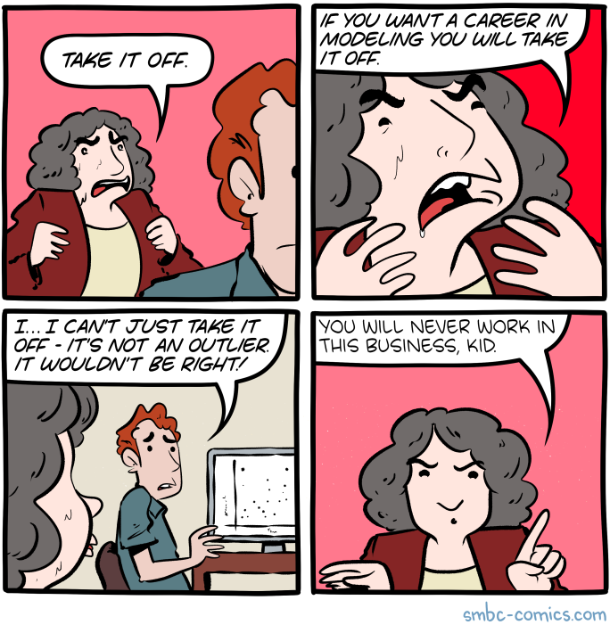
Gaming Statistics with Outliers

SMBC: Take It Off
Anscombe’s Quartet Illustrates Problems With \(R^2\)
Anscombe’s Quartet (Anscombe, 1973) consists of datasets which have the same summary statistics (including \(R^2\)) but very different graphs.

Source: Wikipedia
Alternatives to \(R^2\)
In pretty much every case where \(R^2\) might be useful, (root) mean squared error ((R)MSE) is better.
More generally, we want to think about measures which capture the skill of a probabilistic prediction.
These are commonly called scoring rules (Gneiting & Katzfuss, 2014).
Key Points and Upcoming Schedule
Key Points (Bias)
- Bias: Discrepancy between expected model output and observations.
- Related to approximation error and underfitting.
- “Simpler” models tend to have higher bias.
- High bias suggests less sensitivity to specifics of dataset.
Key Points (Variance)
- Variance: How much the model predictions vary around the mean.
- Related to estimation error and overfitting.
- “More complex” models tend to have higher variance.
- High variance suggests high sensitivity to specifics of dataset.
Key Points (Bias-Variance Tradeoff)
- Error can be decomposed into bias, variance, and irreducible error.
- “Tradeoff” reflects this decomposition (but it’s not really a tradeoff).
- Useful conceptual to think about the balance between not picking up on meaningful signals (underfitting) and modeling noise (overfitting).
Next Classes
Next Week: Model Comparison Methods: Cross-Validation and Information Criteria
Assessments
Project Proposal: Due Friday.
HW4: Will release this week, due 4/11 (after break).
Literature Critique: Talk to Prof. Srikrishnan if you want help finding a paper.
No quiz this week so you can focus on your project proposal.