Scoring and Cross-Validation
Lecture 17
March 24, 2024
Last Class
Bias vs. Variance
- Bias is error from mismatches between the model predictions and the data (\(\text{Bias}[\hat{f}] = \mathbb{E}[\hat{f}] - y\)).
- Variance is error from over-sensitivity to small fluctuations in training inputs \(D\) (\(\text{Variance} = \text{Var}_D(\hat{f}(x; D)\)).
Commonly discussed in terms of “bias-variance tradeoff”: more valuable to think of these as contributors to total error.
Overfitting and Underfitting
- Underfitting: Model predicts individual data points poorly, high bias, think approximation error
- Overfitting: Model generalizes poorly, high variance, think estimation error.
Model Degrees of Freedom
Potential to overfit vs. underfit isn’t directly related to standard metrics of “model complexity” (number of parameters, etc).
Instead, think of degrees of freedom: how much flexibility is there given the model parameterization to “chase” reduced model error?
Regularization
Can reduce degrees of freedom with regularization: tighter/more skeptical priors, shrinkage of estimates (e.g. LASSO) vs. “raw” MLE.
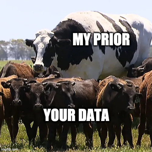
Source: Richard McElreath
Quantifying Prediction Skill
What Makes A Good Prediction?
What do we want to see in a probabilistic projection \(F\)?
- Calibration: Does the predicted CDF \(F(y)\) align with the “true” distribution of observations \(y\)? \[\mathbb{P}(y \leq F^{-1}(\tau)) = \tau \qquad \forall \tau \in [0, 1]\]
- Dispersion: Is the concentration (variance) of \(F\) aligned with the concentration of observations?
- Sharpness: How concentrated are the forecasts \(F\)?
Probability Integral Transform (PIT)
Common to use the PIT to make these more concrete: \(Z_F = F(y)\).
The forecast is probabilistically calibrated if \(Z_F \sim Uniform(0, 1)\).
The forecast is properly dispersed if \(\text{Var}(Z_F) = 1/12\).
Sharpness can be measured by the width of a particular prediction interval. A good forecast is a sharp as possible subject to calibration (Gneiting et al., 2007).
PIT Example: Well-Calibrated
Code
# "true" observation distribution is N(2, 0.5)
obs = rand(Normal(2, 0.5), 50)
# forecast according to the "correct" distribution and obtain PIT
pit_corr = cdf(Normal(2, 0.45), obs)
p_corr = histogram(pit_corr, bins=10, label=false, xlabel=L"$y$", ylabel="Count", size=(500, 500))

xrange = 0:0.01:5
p_cdf1 = plot(xrange, cdf.(Normal(2, 0.4), xrange), xlabel=L"$y$", ylabel="Cumulative Density", label="Forecast", size=(500, 500))
plot!(p_cdf1, xrange, cdf.(Normal(2, 0.5), xrange), label="Truth")

display(p_cdf1)
display(p_corr)PIT Example: Underdispersed
Code
# forecast according to an underdispersed distribution and obtain PIT
pit_under = cdf(Normal(2, 0.1), obs)
p_under = histogram(pit_under, bins=10, label=false, xlabel=L"$y$", ylabel="Count", size=(500, 500))

xrange = 0:0.01:5
p_cdf2 = plot(xrange, cdf.(Normal(2, 0.1), xrange), xlabel=L"$y$", ylabel="Cumulative Density", label="Forecast", size=(500, 500))
plot!(p_cdf2, xrange, cdf.(Normal(2, 0.5), xrange), label="Truth")

display(p_cdf2)
display(p_under)PIT Example: Overdispersed
Code
# forecast according to an overdispersed distribution and obtain PIT
pit_over = cdf(Normal(2, 1), obs)
p_over = histogram(pit_over, bins=10, label=false, xlabel=L"$y$", ylabel="Count", size=(500, 500))

xrange = 0:0.01:5
p_cdf3 = plot(xrange, cdf.(Normal(2, 1), xrange), xlabel=L"$y$", ylabel="Cumulative Density", label="Forecast", size=(500, 500))
plot!(p_cdf3, xrange, cdf.(Normal(2, 0.5), xrange), label="Truth")

display(p_cdf3)
display(p_over)Scoring Rules
Scoring rules compare observations against an entire probabilistic forecast.
A scoring rule \(S(F, y)\) measures the “loss” of a predicted probability distribution \(F\) once an observation \(y\) is obtained.
Typically oriented so smaller = better.
Scoring Rule Examples
- Logarithmic: \(S(F, y) = -\log F(y)\)
- Quadratic (Brier): \(S(F, y) = -2F(y) - \int_{-\infty}^\infty F^2(z) dz\) / \(B(F, y) = \sum_i (y_i - F(y_i))^2\)
- Continous Ranked Probability Score (CRPS): \[\begin{align*} S(F, y) &= -\int (F(z) - \mathbb{I}(y \leq z))^2 dz \\ &= \mathbb{E}_F |Y -y| - \frac{1}{2} E_F | Y - Y'| \end{align*}\]
Proper Scoring Rules
Proper scoring rules are intended to encourage forecasters to provide their full (and honest) forecasts.
Minimized when the forecasted distribution matches the observed distribution:
\[\mathbb{E}_Y(S(G, G)) \leq \mathbb{E}_Y(S(F, G)) \qquad \forall F.\]
It is strictly proper if equality holds only if \(F = G\).
Sidenote: Why Not Use Classification Accuracy?
Most classification algorithms produce a probability (e.g. logistic regression) of different outcomes.
A common skill metric for classification models is accuracy (sensitivity/specificity): given these probabilities and some threshold to translate them into categorical prediction.
The Problem With Classification Accuracy
The problem: This translation is a decision problem, not a statistical problem. A probabilistic scoring rule over the predicted probabilities more accurately reflects the skill of the statistical model.
Logarithmic Score As Scoring Rule
The logarithmic score \(S(F, y) = -\log F(y)\) is (up to equivalence) the only local strictly proper scoring rule (locality ⇒ score depends only on the observation).
This is the negative log-probability: straightforward to use for the likelihood (frequentist forecasts) or posterior (Bayesian forecasts) and generalizes MSE.
We will focus on the logarithmic score.
Important Caveat
A model can predict well without being “correct”!
For example, model selection using predictive criteria does not mean you are selecting the “true” model.
The causes of the data cannot be found in the data alone.
Cross-Validation
Can We Drive Model Error to Zero?
Effectively, no. Why?
- Inherent noise: even a perfect model wouldn’t perfectly predict observations.
- Model mis-specification (the cause of bias)
- Model estimation is never “right” (the cause of variance)
Quantifying Generalization Error
The goal is then to minimize the generalized (expected) error:
\[\mathbb{E}\left[L(X, \theta)\right] = \int_X L(x, \theta) \pi(x)dx\]
where \(L(x, \theta)\) is an error function capturing the discrepancy between \(\hat{f}(x, \theta)\) and \(y\).
In-Sample Error
Since we don’t know the “true” distribution of \(y\), we could try to approximate it using the training data:
\[\hat{L} = \min_{\theta \in \Theta} L(x_n, \theta)\]
But: This is minimizing in-sample error and is likely to result an optimistic score.
Held Out Data
Instead, let’s divide our data into a training dataset \(y_k\) and testing dataset \(\tilde{y}_l\).
- Fit the model to \(y_k\);
- Evaluate error on \(\tilde{y}_l\).
This results in an unbiased estimate of \(\hat{L}\) but is noisy.
\(k\)-Fold Cross-Validation
What if we repeated this procedure for multiple held-out sets?
- Randomly split data into \(k = n / m\) equally-sized subsets.
- For each \(i = 1, \ldots, k\), fit model to \(y_{-i}\) and test on \(y_i\).
If data are large, this is a good approximation.
Leave-One-Out Cross-Validation (LOOCV)
The problem with \(k\)-fold CV, when data is scarce, is withholding \(n/k\) points.
LOO-CV: Set \(k=n\)
The trouble: estimates of \(L\) are highly correlated since every two datasets share \(n-2\) points.
The benefit: LOO-CV approximates seeing “the next datum”.
LOO-CV Algorithm
- Drop one value \(y_i\).
- Refit model on rest of data \(y_{-i}\).
- Predict dropped point \(p(\hat{y}_i | y_{-i})\).
- Evaluate score on dropped point (\(-\log p(y_i | y_{-i})\)).
- Repeat on rest of data set.
LOO-CV Example
Model: \[D \rightarrow S \ {\color{purple}\leftarrow U}\] \[S = f(D, U)\]
LOO-CV Flow
- Drop one value \(y_i\).
- Refit model on \(y_{-i}\).
- Predict \(p(\hat{y}_i | y_{-i})\).
- Evaluate \(-\log p(y_i | y_{-i})\).
- Repeat on rest of data set.
LOO-CV Flow
- Drop one value \(y_i\).
- Refit model on \(y_{-i}\).
- Predict \(p(\hat{y}_i | y_{-i})\).
- Evaluate \(-\log p(y_i | y_{-i})\).
- Repeat on rest of data set.
LOO-CV Flow
- Drop one value \(y_i\).
- Refit model on \(y_{-i}\).
- Predict \(p(\hat{y}_i | y_{-i})\).
- Evaluate \(-\log p(y_i | y_{-i})\).
- Repeat on rest of data set.
Out of Sample:
\(p(y_i | y_{-i})\) = 5.2
In Sample:
\(p(\hat{y}_{-i} | y_{-i})\) = 5.7
LOO-CV Flow
- Drop one value \(y_i\).
- Refit model on \(y_{-i}\).
- Predict \(p(\hat{y}_i | y_{-i})\).
- Evaluate \(-\log p(y_i | y_{-i})\).
- Repeat on rest of data set.
LOO-CV Score: 5.8
This is the average log-likelihood of out-of-sample data.
Bayesian LOO-CV
Bayesian LOO-CV involves using the posterior predictive distribution
\[\begin{align*} \text{lppd}_\text{cv} &= \sum_{i=1}^N \log p_{\text{post}}(y_i | \theta_{-i}) \\ &\approx \sum_{i=1}^N \frac{1}{S} \sum_{s=1}^S log p_{\text{post}}(y_i | \theta_{-i, s}), \end{align*}\]
which requires refitting the model without \(y_i\) for every data point.
Leave-\(k\)-Out Cross-Validation
Drop \(k\) values, refit model on rest of data, check for predictive skill.
As \(k \to n\), this reduces to the prior predictive distribution \[p(y^{\text{rep}}) = \int_{\theta} p(y^{\text{rep}} | \theta) p(\theta) d\theta.\]
Cross-Validation and Model Tuning
Can use cross-validation to evaluate overfitting instead of using different model structure.
What happens to CV error with tighter priors/regularization penalty?
But remember, prediction is not the same as scientific inference: try to balance both considerations.
Challenges with Cross-Validation
- This can be very computationally expensive!
- We often don’t have a lot of data for calibration, so holding some back can be a problem.
- Can have a negative bias for future prediction.
- How to divide data with spatial or temporal structure? This can be addressed by partitioning the data more cleverly: \[y = \{y_{1:t}, y_{-((t+1):T)}\}\] but this makes the data problem worse.
Key Points and Upcoming Schedule
Key Points (Scoring Rules)
- Probabilistic forecasts should be assessed based on both calibration and sharpness.
- Scoring rules as measures of probabilistic forecast skill.
- Logarithmic score (negative log-probability) is the unique locally proper scoring rule.
Key Points (Cross-Validation)
- Gold standard for predictive skill assessment.
- Hold out data (one or more points) randomly, refit model, and quantify predictive skill.
- LOO-CV maximizes use of data but can be computationally expensive.
Next Classes
Wednesday: Entropy and Information Criteria
Assessments
HW4: Due on 4/11 at 9pm.
References
References (Scroll for Full List)
Gneiting, T., Fadoua Balabdaoui, & Raftery, A. E. (2007). Probabilistic Forecasts, Calibration and Sharpness. J. R. Stat. Soc. Series B Stat. Methodol., 69, 243–268. Retrieved from http://www.jstor.org/stable/4623266