import Pkg
Pkg.activate(@__DIR__)
Pkg.instantiate()Homework 1: Thinking About Data
BEE 4850/5850
You can find a Jupyter notebook, data, and a Julia 1.10.x environment in the homework’s Github repository. You should feel free to clone the repository and switch the notebook to another language, or to download the relevant data file(s) and solve the problems creating your own notebook or without using a notebook at all. In either of these cases, if you using a different environment, you will be responsible for setting up an appropriate package environment.
Regardless of your solution method, make sure to include your name and NetID on your solution PDF for submission to Gradescope.
Overview
Instructions
The goal of this homework assignment is to introduce you to simulation-based data analysis.
- Problem 1 asks you to find an example of a spurious correlation.
- Problem 2 asks you to explore whether a difference between data collected from two groups might be statistically meaningful or the result of noise. This problem repeats the analysis from Statistics Without The Agonizing Pain by John Rauser (which is a neat watch!).
- Problem 3 asks you to explore the impacts of selection biases on statistical relationships.
- Problem 4 asks you to evaluate an interview method for finding the level of cheating on a test to determine whether cheating was relatively high or low. This problem was adapted from Bayesian Methods for Hackers.
- Problem 5 (only required for students in BEE 5850) asks you to propose several causal models for the same observational phenomenon.
Load Environment
The following code loads the environment and makes sure all needed packages are installed. This should be at the start of most Julia scripts.
The following packages are included in the environment (to help you find other similar packages in other languages). The code below loads these packages for use in the subsequent notebook (the desired functionality for each package is commented next to the package).
using Random # random number generation and seed-setting
using DataFrames # tabular data structure
using CSVFiles # reads/writes .csv files
using Distributions # interface to work with probability distributions
using Plots # plotting library
using StatsBase # statistical quantities like mean, median, etc
using StatsPlots # some additional statistical plotting tools
Problems
Scoring
Each problem is worth 5 points.
Problem 1
Find an example of a spurious correlation (don’t just pull from Spurious Correlations!!).
In this problem:
- Describe and illustrate the correlation;
- Explain why you think the correlation is spurious.
Problem 2
The underlying question we would like to address is: what is the influence of drinking beer on the likelihood of being bitten by mosquitoes? There is a mechanistic reason why this might occur: mosquitoes are attracted by changes in body temperature and released CO2, and it might be that drinking beer induces these changes. We’ll analyze this question using (synthetic) data which separates an experimental population into two groups, one which drank beer and the other which drank only water.
First, we’ll load data for the number of bites reported by the participants who drank beer. This is in a comma-delimited file, data/bites.csv (which is grossly overkill for this assignment). Each row contains two columns: the group (beer and water) the person belonged to and the number of times that person was bitten.
In Julia, we can do this using CSVFiles.jl, which will read in the .csv file into a DataFrame, which is a typical data structure for tabular data (and equivalent to a Pandas DataFrame in Python or a dataframe in R).
data = DataFrame(load("data/bites.csv")) # load data into DataFrame

# print data variable (semi-colon suppresses echoed output in Julia, which in this case would duplicate the output)
@show data;
How can we tell if there’s a meaningful difference between the two groups? Naively, we might just look at the differences in group means.
Broadcasting
The subsetting operations in the below code use .==, which “broadcasts” the element-wise comparison operator == across every element. The decimal in front of == indicates that this should be used element-wise (every pair of elements compared for equality, returning a vector of true or false values); otherwise Julia would try to just check for vector equality (returning a single true or false value).
Broadcasting is a very specific feature of Julia, so this syntax would look different in a different programming language.
# split data into vectors of bites for each group
beer = data[data.group .== "beer", :bites]
water = data[data.group .== "water", :bites]

observed_difference = mean(beer) - mean(water)
@show observed_difference;
observed_difference = 4.37777777777778This tells us that, on average, the participants in the experiment who drank beer were bitten approximately 4.4 more times than the participants who drank water! Does that seem like a meaningful difference, or could it be the result of random chance?
We will use a simulation approach to address this question, as follows.
- Suppose someone is skeptical of the idea that drinking beer could result in a higher attraction to mosquitoes, and therefore more bites. To this skeptic, the two datasets are really just different samples from the same underlying population of people getting bitten by mosquitoes, rather than two different populations with different propensities for being bitten. This is the skeptic’s hypothesis, versus our hypothesis that drinking beer changes body temperature and CO2 release sufficiently to attract mosquitoes.
- If the skeptic’s hypothesis is true, then we can “shuffle” all of the measurements between the two datasets and re-compute the differences in the means. After repeating this procedure a large number of times, we would obtain a distribution of the differences in means under the assumption that the skeptic’s hypothesis is true.
- Comparing our experimentally-observed difference to this distribution, we can then evaluate the consistency of the skeptic’s hypothesis with the experimental results.
Why Do We Call This A Simulation-Based Approach?
This is a simulation-based approach because the “shuffling” is a non-parametric way of generating new samples from the underlying distribution (more on this later!).
The alternative to this approach is to use a statistical test, such as a t-test, which may have other assumptions which may not be appropriate for this setting, particularly given the seemingly small sample sizes.
In this problem:
- Conduct the above procedure to generate 50,000 simulated datasets under the skeptic’s hypothesis.
- Plot a histogram of the results and add a dashed vertical line to show the experimental difference (if you are using Julia, feel free to look at the Making Plots with Julia tutorial on the class website).
- Draw conclusions about the plausibility of the skeptic’s hypothesis that there is no difference between groups. Feel free to use any quantitative or qualitative assessments of your simulations and the observed difference.
Problem 3
A scientific funding agency receives 200 proposals in response to a call. The panel is asked to evaluate each proposal on two criteria: scientific rigor and potential impact (or “newsworthiness”). After standardizing each of these scores to independently follow a standard normal distribution (\(\text{Normal}(0, 1)\)), the two standardized scores are summed to get the total score for the proposal. Based on these total scores, the top 10% of the proposals are selected for funding.
A researcher who is studying the relationship between rigor and impact has used data on the funded proposals to claim high-impact proposals are necessarily less rigorous, and indeed found a statistically significant negative correlation between the rigor and impact scores for the funded proposals. You are more skeptical and believe this effect is an artifact from the selection process, which would make the claim a bit ironic.
In this problem:
- Create a generative model for the grant-selection procedure under the null assumption of no correlation between rigor and impact. You can sample rigor and impact scores directly from \(\text{Normal}(0, 1)\).
- Using 1,000 simulations, compare the distribution of correlations between rigor and impact for the funded proposals to the general proposal population.
- Explain why, when conditioning on selection for funding, there might be a negative correlation between rigor and impact even when none generally exists.
Selection-Distortion Effects
These selection-distortion effects are pretty common in observational data, going back to work by Dawes in the 1970s on the lack of predictive ability of admission variables on student success and including studies claiming to identify a causal fingerprint of genes on outcomes.
This is, of course, just one example of how not thinking carefully about data-generating processes can fundamentally contaminate statistical analyses, emphasizing that data do not have meaning absent a model for how they were generated.
Problem 4
You are trying to detect how prevalent cheating was on an exam. You are skeptical of the efficacy of just asking the students if they cheated. You are also concerned about privacy — your goal is not to punish individual students, but to see if there are systemic problems that need to be addressed. Someone proposes the following interview procedure, which the class agrees to participate in:
Each student flips a fair coin, with the results hidden from the interviewer. The student answers honestly if the coin comes up heads. Otherwise, if the coin comes up tails, the student flips the coin again, and answers “I did cheat” if heads, and “I did not cheat”, if tails.
We have a hypothesis that cheating was not prevalent, and the proportion of cheaters was no more than 5% of the class; in other words, we expect 5 “true” cheaters out of a class of 100 students. Our TA is more jaded and thinks that cheating was more rampant, and that 30% of the class cheated. The proposed interview procedure is noisy: the interviewer does not know if an admission means that the student cheated, or the result of a heads. However, it gives us a data-generating process that we can model and analyze for consistency with our hypothesis and that of the TA.
In this problem:
- Derive and code a simulation model for the above interview procedure given the “true” probability of cheating \(p\).
- Simulate your model (for a class of 100 students) 50,000 times under a null hypothesis of no cheating, your hypothesis of 5% cheating, the TA’s hypothesis of 30% cheating, and plot the resulting datasets.
- If you received 31 “Yes, I cheated” responses while interviewing your class, what could you conclude?
- How useful do you think the interview procedure is to identify systemic cheating? What changes to the design might you make?
Problem 5
This problem is only required for students in BEE 5850.
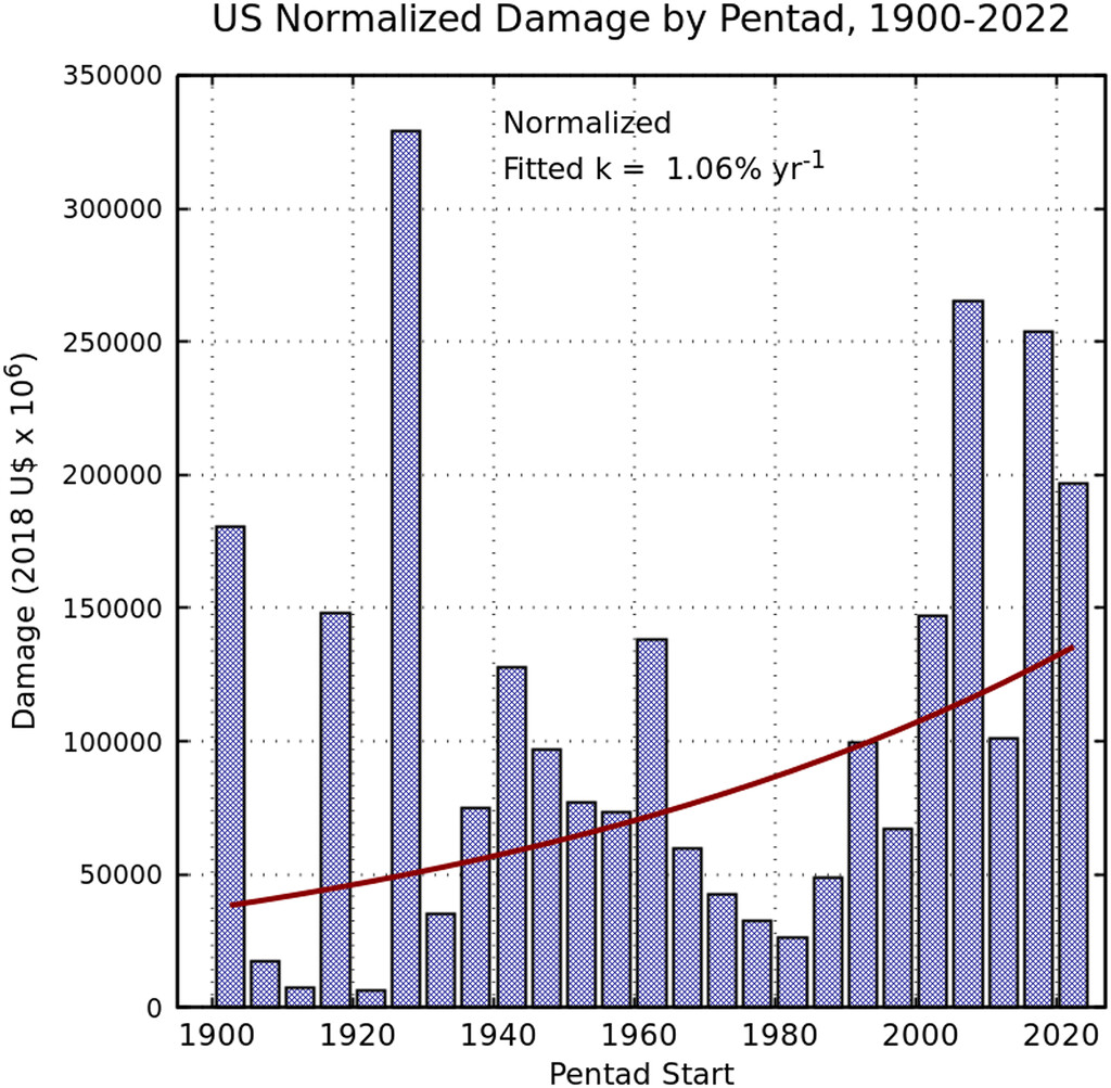
Adjusting for inflation, there has been an increase in tropical cyclone damages on the U.S. Atlantic coast between 1900 and 2022 (see Figure 1).
In this problem:
- Describe two different mechanisms by which tropical cyclone damages in coastal counties might have increased over this period.
- How might you propose to examine the relative strengths of these mechanisms? You don’t need to actually do this (this is indeed a somewhat thorny debate in the literature), but think about potential modeling and data approaches.